Week 7 - Auto ignition using Cantera

Auto ignition using Cantera

Aim

In this challenge, we will work on auto ignition using cantera by performing the following:

• To use the same reactor network code as shown in the video to simulate the Auto Ignition Time for Methane under the following conditions:
  • To plot the variation of Auto Ignition time of Methane with a constant temperature of 1250 K and pressure varying from 1 atm to 5 atm
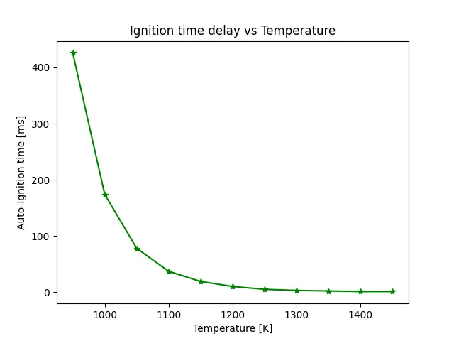
  • To plot the variation of Auto Ignition time of Methane with a constant pressure of 5atm and temperature varying from 950K to 1450K

Theory

Cantera

• Cantera is an open-source suite of tools for problems involving chemical kinetics, thermodynamics, and transport processes.
• Cantera automates the chemical kinetic, thermodynamic, and transport calculations so that the users can efficiently incorporate detailed chemical thermo-kinetics and transport models into their calculations.
• Cantera utilizes object-oriented concepts for robust yet flexible phase models, and algorithms are generalized so that users can explore different phase models with minimal changes to their overall code.
• Cantera can be used from Python and Matlab, or in applications written in C/C++ and Fortran 90.
• Cantera is currently used for applications including combustion, detonations, electrochemical energy conversion and storage, fuel cells, batteries, aqueous electrolyte solutions, plasmas, and thin film deposition.
• Cantera Reactor relates to a large thermodynamic control volume with uniform distribution of all state variables.
• The system is inherently unstable, in the sense that all states are time-dependent. Chemical processes, in particular, can cause transitory state shifts. Thermodynamic equilibrium, on the other hand, is believed to exist throughout the reactor at all times.

Reactors can interact with their surroundings in a variety of ways:

• Expansion/compression work by using the volume of the reactor
• Heat transfer across the reactor's boundaries
• The reactor can have several inlets and outputs for mass transfer.
• Surface interaction by mass transfer between the surface and the fluid may also be represented

Governing equations in reactors

-> Conservation of mass

i.e `(dm)/(dt)=sum_(In)m_(In)^. - sum_(out)m_(out)^. + m_(wall)^.`

-> Conservation of species

`(dY_k)/(dt)=sum_(In)m_(In)^.(Y_(kIn)-Y_(Kout)) + m_(k)^.`

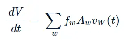
-> Reactor volume

-> Conservation of energy

Types of reactor model

->Constant pressure model

• For this reactor model, the pressure is held constant.
• The volume is not a state variable, but instead takes on whatever value is consistent with holding the pressure constant.
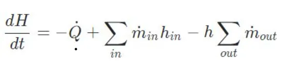
• The total enthalpy replaces the total internal energy as a state variable. Using the definition of the total enthalpy:

`H=U+PV`

`(dH)/dt=(dU)/dt +P(dV)/dt +V(dP)/dt`

Applying dp/dt=0 and substituting into the energy eqn, the above eqn yields

Code

• The code starts with necessary libraries and then the gas object is defined from the concepts of object oriented programming.
• The temperature of gas is assumed to be at 1250 K and then we write the start time and end time parameters in the subsequent lines of the program.
• The program is run for 10 seconds with a time step of 1ms or 1e-3 seconds.
• Now since the pressure is to be varied from 1 bar to 5 bar, the linspace command defines 9 values of pressure.
• Then we are appending the states object by defining the convergence loop of error. The results are then plotted as shown below

A code is written in python by importing cantera, matplotlib and numpy and the videos are followed for writing the code as shown below:

import matplotlib.pyplot as plt 
import cantera as ct 
import numpy as np 

gas = ct.Solution('gri30.xml')
Pressure = np.linspace(1,5,9)
Temperature_intial = 1250
time_start = 0.0
time_end = 10.0
time_step = 1e-3
n = int((time_end - time_start)/time_step)
time_autoIgnition_Pressure = []
states1 =[]

for i in Pressure:
	gas.TPX = Temperature_intial, i*101325,{'CH4' : 1, 'O2':2, 'N2':7.52}
	Temperature_autoIgnition = 0
	time_autoIgnition = 0
	time = 0
	r = ct.IdealGasReactor(gas)
	sim = ct.ReactorNet([r])
	states = ct.SolutionArray(gas,extra = ['time_in_ms','t'])
	print('{:10s} {:10s} {:10s}'.format('t[s]','T[K]','P[Pa]'))

	for j in range(n) : 
		time += 1e-3
		sim.advance(time)
		states.append(r.thermo.state,time_in_ms = time*1e3,t=time)
		

	states1.append(states.T)
	
	for i in range(n):
		Temperature_error = states.T[i] - Temperature_intial - 400
		if Temperature_error >0:
			Temperature_autoIgnition = states.T[i]
			time_autoIgnition = states.time_in_ms[i]
			break
	time_autoIgnition_Pressure.append(time_autoIgnition)

states1 = np.array(states1)

for k in range(len(Pressure)):
	plt.figure(1)
	plt.plot(states1[k])
	plt.xlabel('Number of timesteps')
	plt.ylabel('Temperature')
	plt.title('Variation of Auto-Ignition Tempetature with inlet pressure')
	plt.legend(['1 Bar','1.5 Bar','2 Bar','2.5 Bar','3 Bar','3.5 Bar','4 Bar','4.5 Bar','5 Bar'])

plt.figure(2)
plt.plot(Pressure,time_autoIgnition_Pressure,'b-*')
plt.xlabel('Pressure [bar]')
plt.ylabel('Auto-Ignition time [ms]')
plt.title('Ignition time delay vs Pressure')
plt.show()

Temperature = np.linspace(950,1450,11)
time_autoIgnition_Temperature = []
states2 = []
for i in Temperature:
	gas.TPX = i, 5*101325,{'CH4' : 1, 'O2':2, 'N2':7.52}
	Temperature_autoIgnition = 0
	time_autoIgnition = 0
	time = 0
	r = ct.IdealGasReactor(gas)
	sim = ct.ReactorNet([r])
	states = ct.SolutionArray(gas,extra = ['time_in_ms','t'])
	

	for j in range(n) : 
		time += 1e-3
		sim.advance(time)
		states.append(r.thermo.state,time_in_ms = time*1e3,t=time)
		

	states2.append(states.T)

	for j in range(n):
		Temperature_error = states.T[j] - Temperature_intial - 400
		if Temperature_error >0:
			Temperature_autoIgnition = states.T[j]
			time_autoIgnition = states.time_in_ms[j]
			break
	time_autoIgnition_Temperature.append(time_autoIgnition)

states2 = np.array(states2)

for m in range(len(Temperature)):
	plt.figure(3)
	plt.plot(states2[m])
	plt.xlabel('Number of timesteps')
	plt.ylabel('Temperature')
	plt.title('Variation of Auto-Ignition Tempetature with inlet pressure')
	plt.legend(['950 K','1000 K','1050 K','1100 K','1150 K','1200 K','1250 K','1300 K','1350 K','1400 K','1450 K'])

plt.figure(4)
plt.plot(Temperature,time_autoIgnition_Temperature,'g-*')
plt.xlabel('Temperature [K]')
plt.ylabel('Auto-Ignition time [ms]')
plt.title('Ignition time delay vs Temperature')
plt.show()

plt.figure(5)
plt.subplot(3,1,1)
plt.plot(states.t,states.X[:,gas.species_index('H2O')])
plt.xlabel('Time (ms)')
plt.ylabel('H2O Mole Fraction')
plt.subplot(3,1,2)
plt.plot(states.t,states.X[:,gas.species_index('O2')])
plt.xlabel('Time (ms)')
plt.ylabel('O2 Mole Fraction')
plt.subplot(3,1,3)
plt.plot(states.t,states.X[:,gas.species_index('OH')])
plt.xlabel('Time (ms)')
plt.ylabel('OH Mole Fraction')
plt.tight_layout()
plt.show()

AutoIg_Temp = [500,1000]
states3 =[]
for i in AutoIg_Temp:
	gas.TPX = i, 5*101325,{'CH4' : 1, 'O2':2, 'N2':7.52}
	r = ct.IdealGasReactor(gas)
	sim = ct.ReactorNet([r])
	time = 0
	states = ct.SolutionArray(gas)

	for n in range(1000):
		time += 1e-3
		sim.advance(time)
		states.append(r.thermo.state)

states3 = np.array(states.T)

plt.figure(6)
plt.plot(states3)
plt.xlabel('Number of timesteps')
plt.ylabel('Temperature')
plt.title('Temperature variation at 500 K & 1000 K')
plt.show()

Results and Discussions

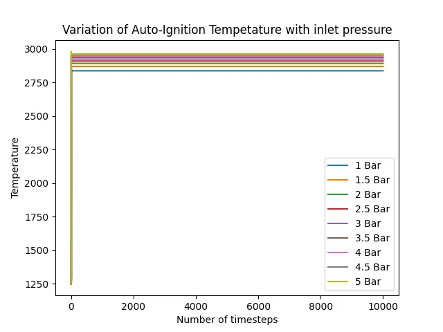
• The above plot shows variation of Auto ignition temperature was the time proceeds by varying the inlet pressure.
• Here we vary the inlet pressure all the way from 1bar to 5bar.
• We can infer that with high inlet pressure, we can attain high temperature in the reactor.
• This is due to the fact that heat addition at higher pressure is more efficient than at low pressure

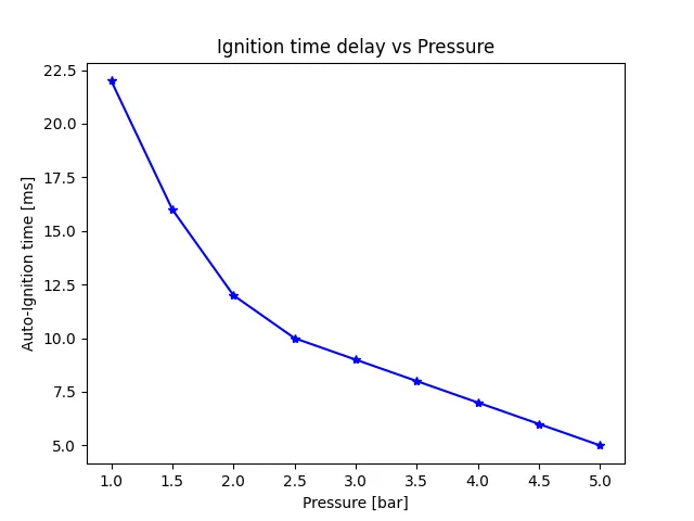
• The above is a plot of ignition time vs pressure.
• It can be seen that as the pressure increases, the time to ignite the mixture decreases.
• This is due to the fact that energy addition at higher pressure is more efficient than at low pressure

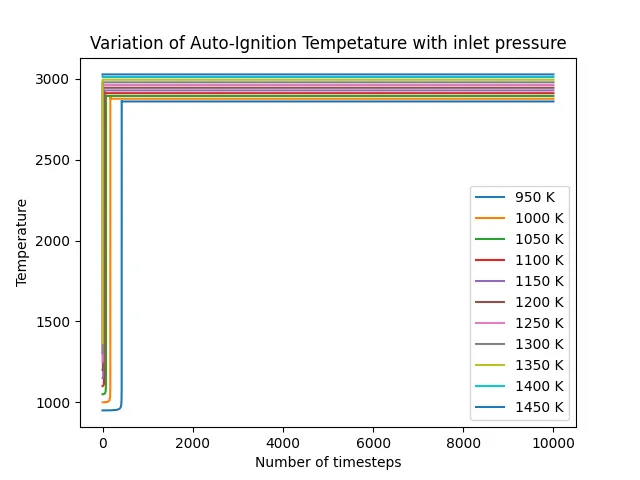
• In this plot, we vary the inlet temperature from 950K to 1450K by keeping the inlet pressure as constant at 5atm.

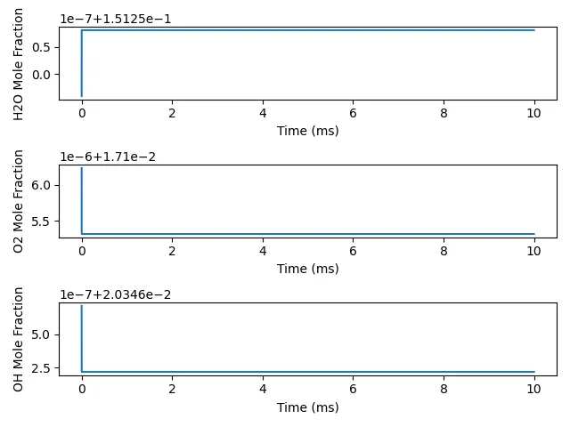
• This is a plot showing the variation of mole fraction of species with time.
• Note that as the reaction proceeds, the concentration of the reaction decreases.
• Hence the mole fraction of the reactants decreases.
• But as the concentration of products increase due to conversion of reactants to products, hence ots molefraction increases.
• In the above case, we see that the concentration of O2 and OH ions decrease as the reaction proceeds whilst the concentration of water increases due to the following reaction
  • `CH_4 +2(O_2+3.76N_2) -> CO_2 + 2H_2O+7.52N_2`

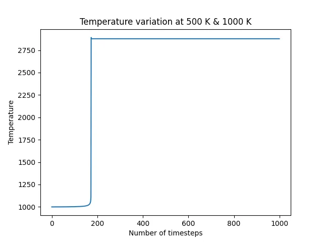
When we add energy to the reactants, it takes some time(of the order of a few microseconds) to ignite the mixture. The above plot shows the increase in the value of temperature as the reaction proceeds.

Thus the Auto ignition delay using cantera is carried out and the plots are shown above and the results are discussed.