Week 5.2 - Literature review: ODE Stability

Literature review: ODE Stability

Aim

In this challenge, we will be working on a literature survey to answer the following questions alongside writing a code that will help us in answering these as follows:

• When does a ODE become unstable?
• How does stability affect engineering simulations?
• Can stability condition be derived for all types of problems?

Theory

Many modeling problems in engineering applications can be formulated using ordinary differential equations. There are a few different definitions of differential equation; one of the simplest ones is “A differential equation is any equation which contains derivatives, either ordinary derivatives or partial derivatives” given in [1]. From this definition, we can derive that there are two types of differential equations: ordinary differential equations (ODEs) and partial differential equations (PDEs). ODEs contain one type of derivative or one independent variable, while PDEs contain two or more derivatives or independent variables. For example, a general form for first-order ODEs can be expressed by:

`(dy)/(dx)=f(x,y)` -[1]

where y(x) is a dependent variable whose values depend on values of the independent variable of x. Another good example of an ODE is Newton’s second law of motion formulated by:

`ma=(dp)/(dt)=(mdv)/(dt)=F(t,v)`

where F(t, v) is the force, which is a function of time (t) and velocity (v);

`(dv)/(dt)`is a velocity change rate (acceleration) of a moving object; m is the mass of a moving object; a is an
acceleration of a moving object; p is momentum; and `(dp)/(dt)`is its derivative.

The previous formulation of Newton’s second law can be also rewritten in the following way:

`m(d/dx((dx)/dt))=m((d^2x)/dt^2)=F(t,x,(dx)/dt)`

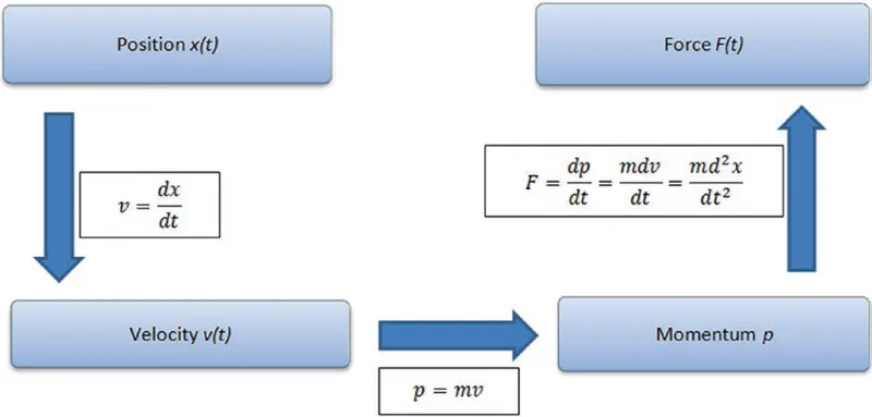
where the derivative `(dx)/dt` of the displacement x of a moving object is the velocity v. In other words, the velocity is a change rate of the displacement x(t) of a moving object in time. This can be visualised as follows:

Classifying ODEs

There are two classifications of ODE-related problems.

• Initial value problems (IVPs)

`x^(..) = xt - 3x^.`with these initial conditions: x(0) = 3, `x^.(0)=1`

• Boundary value problems (BVPs):

`x^(..) = xt - 3x^.` with these boundary conditions: x(0) = 3, x(2) = 1.50.

IVPs are defined with ODEs together with a specified value, called the initial condition, of the unknown function at a given point in the solution domain. In the IVP of ODEs, there might be a unique solution, no solution, or many solutions. By definition,the IVP of ODEs can be explicitly defined or implicitly defined. Most IVPs are explicitly
defined.

Coding Logic and Procedure

• The logic is to solve a differential equation `dy/dt=-1000*y-e^(-t)`
• To solve this we will follow two system of approaches-explicit and implicit.
• Explicit and implicit methods are approaches used in numerical analysis for obtaining numerical approximations to the solutions of time-dependent ordinary and partial differential equations, as is required in computer simulations of physical processes.
• Explicit methods calculate the state of a system at a later time from the state of the system at the current time, while implicit methods find a solution by solving an equation involving both the current state of the system and the later one.
• Mathematically, if is the current system state and is the state at the later time is a small time step), then, for an explicit method

while for an implicit method one solves an equation

to find

• Once done, we will declare the time array and vary the timestep size.
• Also, we will declare an initial set of solution matrix. Once done, the program runs and then the results are visualised.

import matplotlib.pyplot as plt
import numpy as np
#to solve ode using euler's forward method

def explicit_solver(total_t,dt):
	t=np.arange(0,total_t,dt)
	y=np.zeros(len(t))

	for i in range(1,len(t)):
		y[i]=y[i-1] - dt*(1000*y[i-1] + np.exp(-t[i-1]))

	return [t, y] 

def implicit_solver(total_t,dt):
	t=np.arange(0,total_t,dt)
	y=np.zeros(len(t))
	#formula to calculate
	for i in range(1,len(t)):
		y[i]=(y[i-1] -np.exp(-t[i-1])*dt)/(1+ 1000*dt)

	return [t, y] 

total_t=0.1;
dt=1e-2
#calling the function
t,y_explicit=explicit_solver(total_t,dt)
t,y_implicit=implicit_solver(total_t,dt)

plt.plot(t,y_explicit,color='red')
plt.plot(t,y_implicit,color='blue')
plt.legend(['Explicit','Implicit'])
plt.title('Timestep size=1e-2 s')
plt.xlabel('total time')
plt.ylabel('Solution')
plt.show()

Results and Discussions

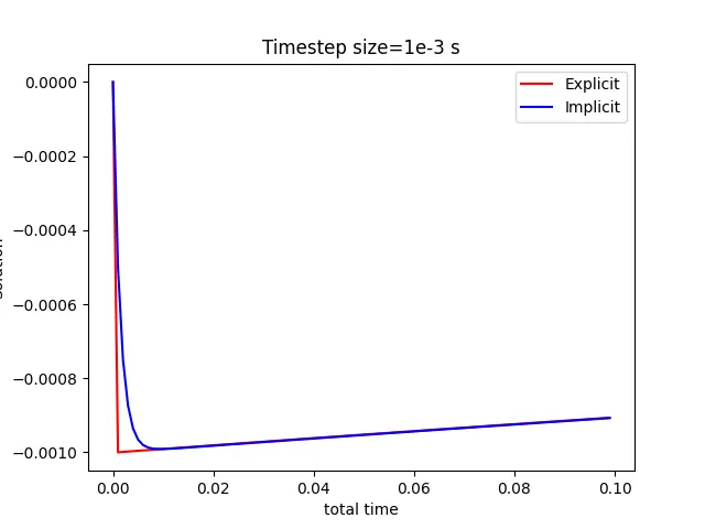
For a time step size of 1e-3 s

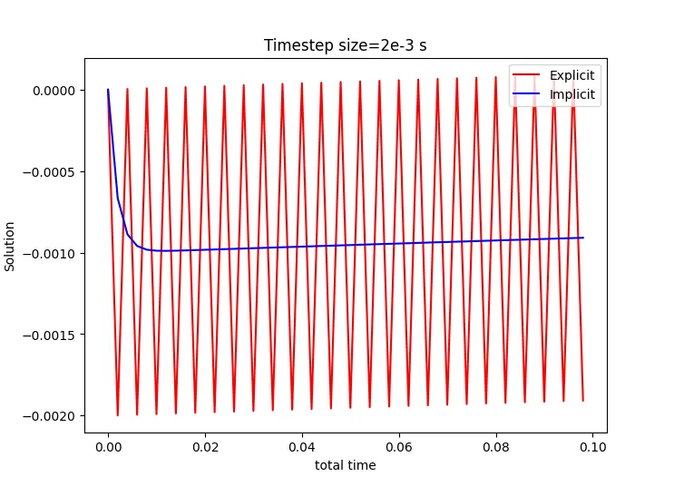
For timestep size of 0.002s

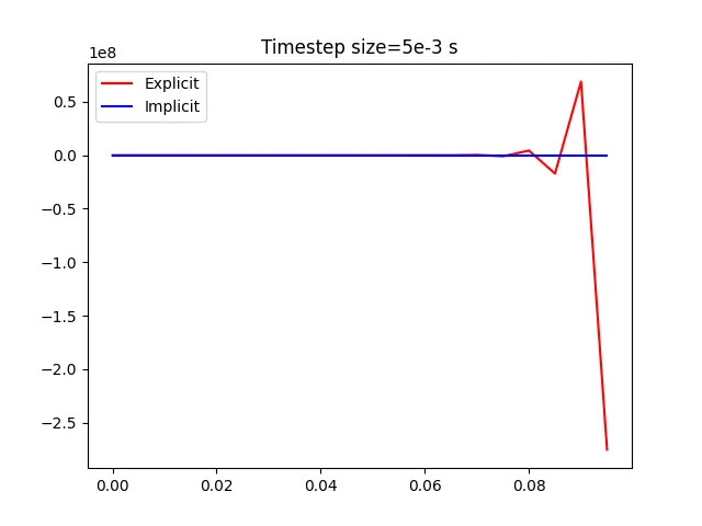
For a timestep size of 0.005 s

For a timestep size of 0.01s

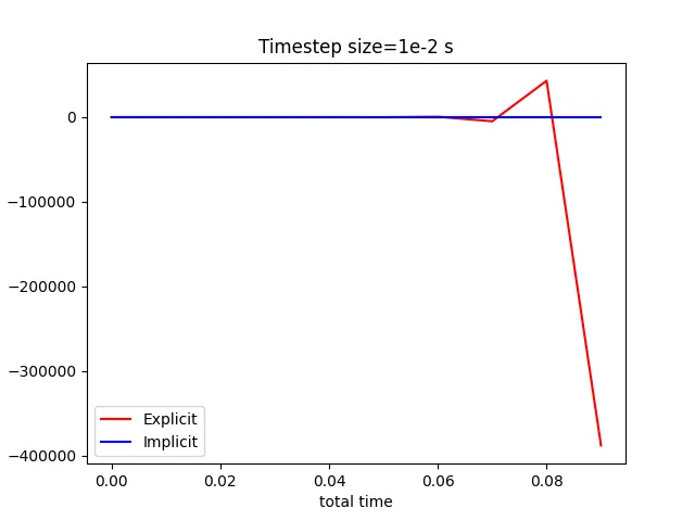
• As can be seen from the above plots, Explicit solution shows a strong step-wise variation at t=0, while implicit solution shows a smooth variation.
• Eventhough the variation in the solution can be considered minimal, this affects the solution when we consider large time scale difference.
• On raising the timestep scale to 0.002s, we can see wild oscillations and fluctuations in the explicit solution, whereas an implicit solution remains almost the same as it was in the previous timestep value.
• Thus we can conclude that upto a certain value of time step size as determined by CFL criterion(unique for a given PDE), explicit and implicit solutons almost remains same.
• Once we increase the timestep size to enormous values, the explicit scheme simply blows up the solution, whereas the implicit solution provides more or less the same answer.
• Thus we can say that the implicit solution is unconditionally stable, whereas the explicit scheme is timestep dependent.
• Stability, in mathematics, condition in which a slight disturbance in a system does not produce too disrupting an effect on that system.
• In terms of the solution of a differential equation, a function f(x) is said to be stable if any other solution of the equation that starts out sufficiently close to it when x = 0 remains close to it for succeeding values of x.
• If the difference between the solutions approaches zero as x increases, the solution is called asymptotically stable. If a solution does not have either of these properties, it is called unstable.
• Stability of solutions is important in physical problems because if slight deviations from the mathematical model caused by unavoidable errors in measurement do not have a correspondingly slight effect on the solution, the mathematical equations describing the problem will not accurately predict the future outcome.
• In the numerical simulations (computational analysis), numerical stability is a generally desirable property. The precise definition of stability depends on the context.
• One is numerical linear algebra and the other is algorithms for solving ordinary and partial differential equations by discrete approximation.
• In numerical linear algebra the principal concern is instabilities caused by proximity to singularities of various kinds, such as very small or nearly colliding eigenvalues.
• On the other hand, in numerical algorithms for differential equations the concern is the growth of round-off errors and/or small fluctuations in initial data which might cause a large deviation of final answer from the exact solution.
• Some numerical algorithms may damp out the small fluctuations (errors) in the input data; others might magnify such errors.
• Calculations that can be proven not to magnify approximation errors are called numerically stable.
• One of the common tasks of numerical analysis is to try to select algorithms which are robust – that is to say, do not produce a wildly different result for very small change in the input data.
• Engineering problems are real life problems and stability plays important role in solution, so if solution for such problem is unstable it will lead in failure of product.
• So it is undesirable and hazardous to have unstable solution in engineering problems.
• Stability in engineering simulations depends on some factors like upwind schemes, solving methods (implicit or explicit), time step size, mesh grid size, relaxation factor, etc.
• For example, while using coarse mesh with fist order upwind scheme, we get converged solution fast (with few number of iterations) but it would not be accurate and stable.
• So for coarse mesh choosing second order scheme is a good choice.
• Second order scheme use a greater number of neighboring cells to computes flow variables at a point, therefore it gives accurate results.
• Using under relaxation factor also helps in giving solution greater stability, though it takes more time in convergence as compared to relaxed or over relaxed system.
• Under relaxation factor prevents oscillation in our results. Another condition is CFL condition or ‘Courant number’, it also affects simulation results. This term gives unstable results if size of our time step is larger than the distance between two neighboring cells in mesh grid. So using correct time step size is very important.

Thus the literature survey has been carried out by writing a code in python.