Week 10: Project 1 - FULL HYDRO case set up (PFI)

Simulation of full hydro setup of a Port Fuel Injection(PFI) engine

In this project, we shall continue the previous project by setting up a full-hydro case setup in converge and post process the results file and visualise the meshing process.

PFI-a look

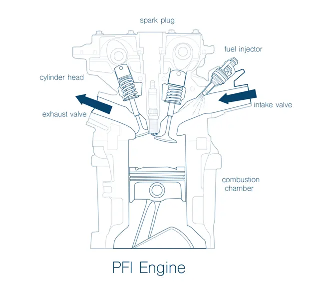
PFI engines use a three-way catalytic converter, exhaust sensors and computer-controlled engine management to constantly adjust the fuel-to-air ratio injected into each cylinder. Since the fuel is injected right before the cylinder, most of the fuel will be drawn into the cylinder causing less collection/stagnation of fuel in the manifold. One other advantage of this type of injection is that, the intake manifolds is not necessary to be made of metal as intake will mostly contain air at atmospheric pressure. This can reduce the weight and overall cost of the engine as well.

Spray modeling

Converge has built in models utilized for spray processes including liquid atomization, drop breakup, collision and coalescence, turbulent dispersion and drop evaporation. These models have mathematical approximations necessary to capture the physics behind the processes mentioned above and the combustion aspect as well.

In IC engines, the fuel is sprayed in the combustion chamber or near intake valves. This fuel spray can be completely simulated using CFD multiphase simulations, but doing so in a IC engine simulation would result in the simulation running for very long. This can be prevented if we statistically model the same effect of the spray instead of actually simulating it. This approximating process of fuel sprays is called Spray modelling. Any fuel spray undergoes a mechanism which has the following processes:

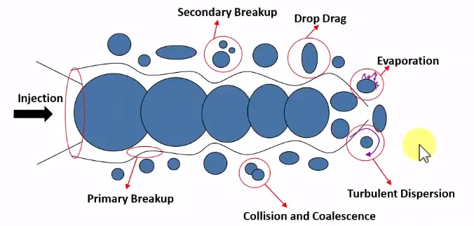
1) Primary Breakup: Splitting of a drop from the mainstream

2) Secondary Breakup: Splitting of a primary drop into multiple drops

3) Drop Drag: Drag caused by air on the moving drop.

4) Collision and coalescence: Collision of two or more drops and formation of the new drop.

5) Turbulent dispersion: Transport of mass, heat, or momentum within a system due to random and chaotic time-dependent motions

6) Evaporation: Evaporation of small liquid drops into vapour

The sequence of processes is easy to understand. The mainstream breaks into multiple drops by primary and secondary breakups. New drops are formed due to coalescence. The evaporation reduces the drops and dispersion spreads the drops into the region. While modelling the spray, each process is represented mathematically by using some pre-established models. These create the effect of spray without actually simulating the spray.

To calculate the spray in a simulation, CONVERGE introduces drop parcels into the domain at the injector location at a user-specified rate. Parcels represent a group of identical drops (i.e., same radius, velocity, temperature, etc.) and are used to statistically represent the entire spray field.

Evaporation: The evaporation is simulated using Frossling or Chiang model. They are responsible for flagging a parcel drop as evaporated or not. They consider the size of the drop and its evaporation properties to make decisions for drops.

Penetration: The fuel spray penetration is also recorded in the software. It calculates this based on how long did the fuel travel as a liquid. The cell up to which the 0.95*(mass of liquid fuel sprayed) is seen is called the liquid penetration length.

Collision: The software contains two models: O'Rourke model and NTC model. These models simulate the collision using a collision grid. Using a collision grid creates accurate particle movement data.

Drop Drag: This is simulated using Spherical drop drag model or Dynamic drop drag model. The Spherical model calculates the drag coefficient based on assuming the shape of drop as the sphere, while the dynamic model accounts for variations in drop shape. It uses TAB model to determine the drop distortion.

Drop wall interaction: When a drop parcel would collide with the wall, it could rebound back, escape or remain on the wall, creating a film. These effects are modelled using: O'Rourke model or Kuhnke model.

CONVERGE offers two categories of liquid injection mechanisms: injectors and nozzles. An injector is a group of nozzles that have some of the same characteristics. Each injector can have any number of nozzles, each with its own hole size, cone angle, position, and orientation.

Injector models: The models used are 'Kelvin-Helmholtz model' and 'Rayleigh-Taylor model'. These models look after the primary and secondary breakup of parcel drops. The calculations are based on 'Kelvin-Helmholtz instability theory' and 'Rayleigh-Taylor instability theory'. These theories are used for surface tension instabilities of the drop, which lead to a fluid breakup.

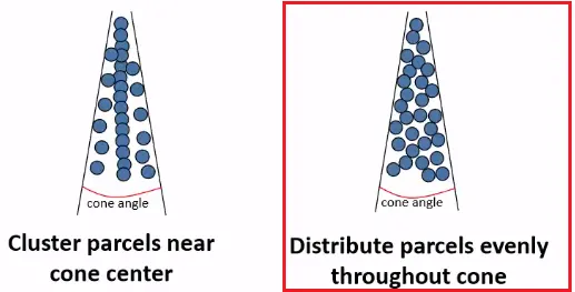
i) General: For solid cone sprays, converge assumes the injection is conical.

• Parcel distribution: Distribute parcels evenly throughout cone.
• 
• Penetration: Converge writes the liquid and vapor penetration lengths at each output interval, it calculates vapor penetration length for each nozzle.

• Liquid fuel mass fraction for calculating spray penetration: 0.95

• Liquid penetration length is the distance that encompasses the calculated penetration spray mass. Converge calculates the penetrated spray mass by multiplying the mass fraction by total liquid mass in the domain.
• Liquid penetration length is not calculated along the spray axis of the nozzle but it is calculated along the injector axis
• Bin size for calculating vapor penetration: 0.001 m
• Providing bin size for calculating the vapor penetration, cell size is at least 2 times smaller than bin size, especially in the location of spray.
• Fuel vapor mass fraction for calculating vapor penetration: 0.001
• Cell, where the vapor is present, have some minimum amount of vapour and that is characterized by "fuel vapour mass fraction for calculating vapour penetration". Its value 0.001 means that particular cell content 1e-3 vapour in terms of mass fraction coma anything less than that can be considered as a cell that not containing vapour.

ii) Collision/Breakup/Drag:

Collision model: NTC collision

Collision outcomes: Post-collision outcomes

Enable collision mesh

• Collision calculation based upon if the one parcel is going to hit the other parcel or not.
• Parcels are Lagrangian parcels have their own space and gas-phase have their own space.
• To perform collision calculation we need another mesh which is different from the original mesh provided. This is called the collision mesh

Collision calculations can be highly grid-sensitive when an underresolved the fluid-phase mesh is used. To help alleviate this issue, the collision mesh option has been implemented in CONVERGE, based on the concept of a collision mesh proposed by Hou. In a simulation without collision mesh, parcels collide only with parcels in the same grid cell. This can lead to artefacts in the spray since parcels do not collide across cell walls. This can also slow down computational time because there can be many parcels in larger cells. Using a collision mesh can eliminate both these problems. Simulations with collision mesh can much more accurately represent the spray dispersion by eliminating grid effects.

Using a collision mesh can eliminate both these problems. Simulations with collision mesh can much more accurately represent the spray dispersion by eliminating grid effects.

An alternative to the O’Rourke numerical collision scheme is the No Time Counter (NTC) method of Schmidt and Rutland. The NTC method is based on techniques used in gas dynamics for Direct Simulation Monte Carlo (DSMC) calculations. This model is faster and more accurate than O’Rourke’s model under certain conditions.
The NTC method involves stochastic (randomly determined) sub-sampling of the parcels within each cell.

This potentially results in much faster collision calculations. Unlike O'Rourke's method, which incurs an additional computational cost that increases with the square of the number of parcels, the NTC method has a linear cost. O'Rourke's method assumes that multiple collisions can occur between parcels and that this process is governed by a Poisson distribution. However, the Poisson distribution is not correct unless collision has no consequences for the parcels. Since collisions change parcels’ velocities, size, and number, the method of repeated sampling used by the NTC method generates more accurate answers (Schmidt and Rutland, 2000). The NTC method is derived, without assumptions, from the basic probability model for the stochastic collision. The basic probability model requires that the cell size is sufficiently small such that spatial variations in spray quantities can be neglected. These assumptions are a subset of those required for deriving the O’Rourke collision mode.

Combustion modelling

Combustion Facilitates the energy transfer in an engine.

The combustion is modelled by using its reaction mechanism. There are multiple species and intermediate reactions which govern the combustion process. The reaction mechanism of real-life combustion is very large and simulating it directly would take a long time. So, the combustion is solved only for those reactions and species whose presence affects the combustion results. This is called a reduced mechanism file. These all processes of reducing mechanism and solving them is done by various solvers present in the software: SAGE, CTC/ Shell, G-Equation, CEQ, FGM, etc. In this report, SAGE solver is used, so details of SAGE are only given.

SAGE: It's a detailed chemistry solver which uses local conditions to calculate the reaction rates based on principles of Chemical kinetics. It calculates the heat release, which is used as a source term in fluid flow energy equations. The species are modelled using chemical kinetics ODEs and the values are used in species transport equations. The Solver used to solve the ODEs is CVODES.

Acceleration technique: The SAGE solver is a detailed chemistry solver, meaning that it would calculate values based on full mechanism instead of reducing it. This takes a lot of time if the calculations are done for every cell in the mesh. So, to increase the speed of solving, the solver is run using a multizone model. All the cells where combustion is going to be solved for, are grouped into bins. The bins are created based on the temperature and equivalence ratio of fuel and air. All the cells having the same temperature and equivalence ratio will have the same combustion results. So, the SAGE solver is solved once for each bin and accordingly the flow and species data is remapped to the cells. This increases the speed tremendously. The bins can also be created based on multiple variables like pressure, reaction ratio, etc.

Procedure

The procedure involves first importing the CAD file into the converge studio, followed by cleaning the geometry. This is achieved by surface preparation of the gometry followed by boundary flagging. Once done, we will setup the case and then run the simulation.

• 
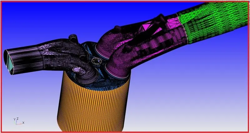
• This is the geometry that looks like after cleaning and marking the boundaries.
• The individual boundaries that are flagged are shown below:
• 
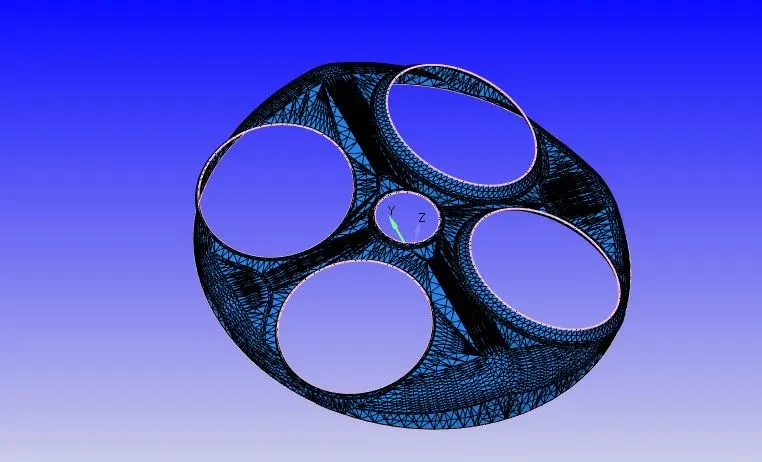
• Cylinder head
• 
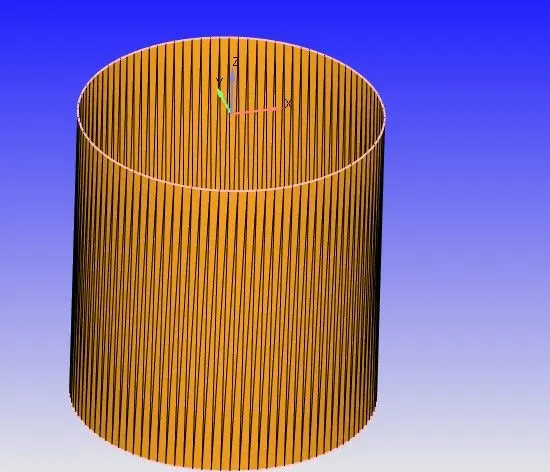
• Liner
• 
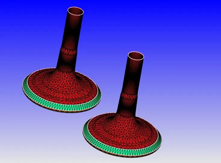
• Exhaust valve
• 
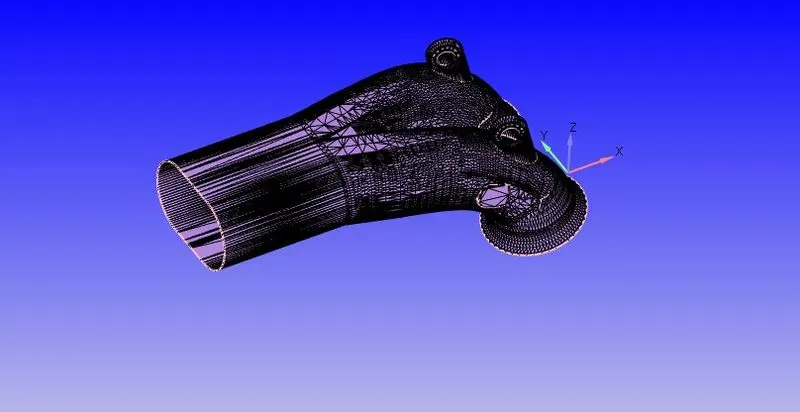
• Exhaust Port
• 
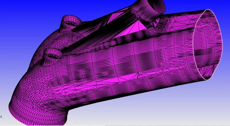
• Intake Port
• 
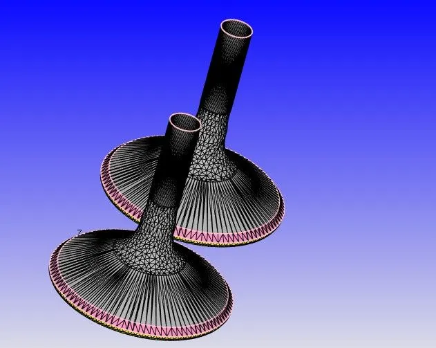
• Intake Valve
• 
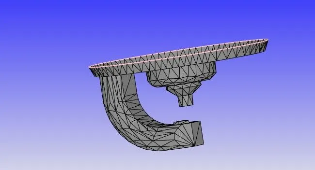
• Spark plug

Once done, lets begin case setup

• Set the application type as IC engine based.
• In the materials, choose the reaction mechanism and turn it on.
• 
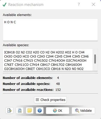
• Import the necessary ".dat" file and click OK.
• 
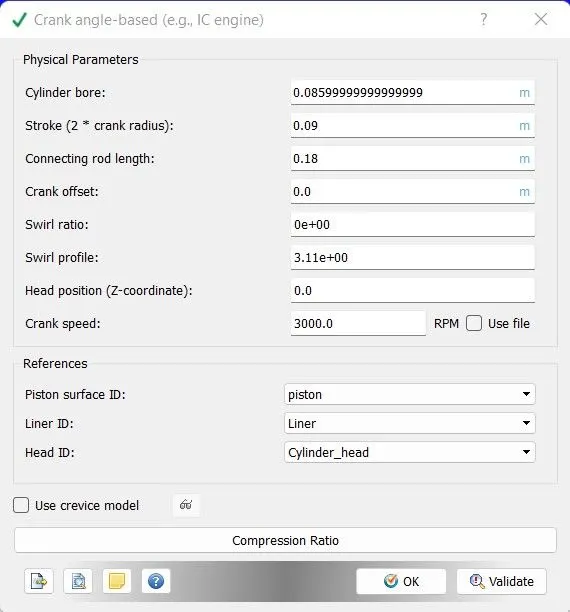
• Enter these parameters as shown above for a crank case engine.
• 
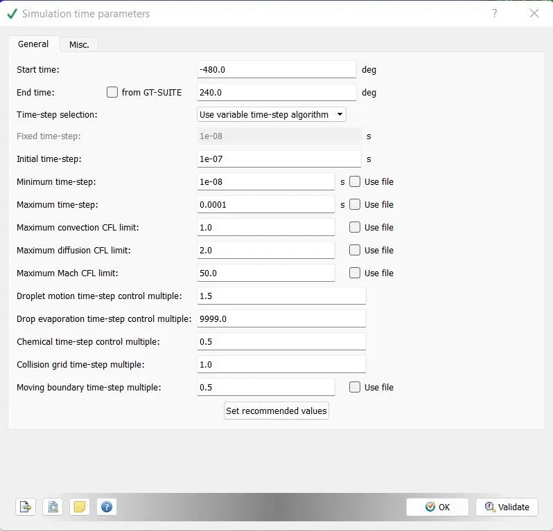
• Enter the time parameters to run the simulation as shown above.
• Once done, create four regions that depict different physical and chemical properties of the flow at different regions as cylinder, intake regions-1 &2 and exhaust region as shown below.
• Calculation of mass fraction of species
• For combustion, we know that the balanced chemical reaction for iso-octane is as follows
• `C_8H_18+a(O_2+3.76*N_2)->CO_2+H_2O+N_2`
• Upon balancing this reaction, we get
• `C_8H_18+12.5(O_2+3.76*N_2)->8CO_2+9H_2O+12.5*3.76N_2`

• Species	Molecular mass	Mass fraction
  `C_8H_18`	114.23	0.025508
  `O_2`	32*12.5	0.20157
  `N_2`	28*12.5*3.76	0.77292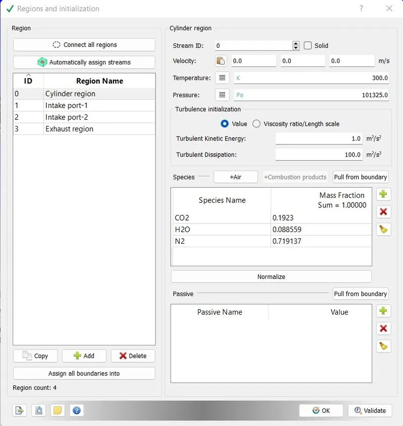

• 
• The intake port-1 is the region closer to the cylinder and thus carries a fuel C8H18">C8H18C8H18with air as follows

• Species	Mass Fractions
  `C_8H_18`	0.025508
  `O_2`	0.20157
  `N_2`	0.77292

• (How these values are provided to be explained)
• The intake port 2 contains only air and hence the air is entered
• The exhaust and the cylinder regions contains the products of combustion viz. `CO_2,H_2O,N_2`with the mass fractions which are specified below:

• Species	Mass Fractions
  `CO_2`	0.1923
  `H_2O`	0.08559
  `N_2`	0.719137

• The temperatures are setup accordingly, as follows:

• Boundary	Temperature
  Piston	450
  Liner	450
  Head	450
  Spark Plug	550
  Spark plug electrode	600
  Exhaust Port	500
  Exhaust Outflow	800
  Exhaust valve(all top, angle,bottom)	525
  Intake valve(all top,angle,bottom)	480
  Intake port(both 1&2)	425
  Inflow temperature	363

• Once done, click on boundary and allot "law of wall" to the boundaries that were alloted the wall BC and for piston,mark the BC as wall with translation motion enabling a piston type motion.
• For intake valve and exhaust valve, import "intake_lift.in" and "exhaust_lift.in" files respectively.
• Once done,create events as shown below:
• 
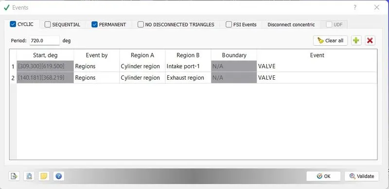
• A cyclic event is setup to simulate valve motion between cylinder regions and intake port-1
• 
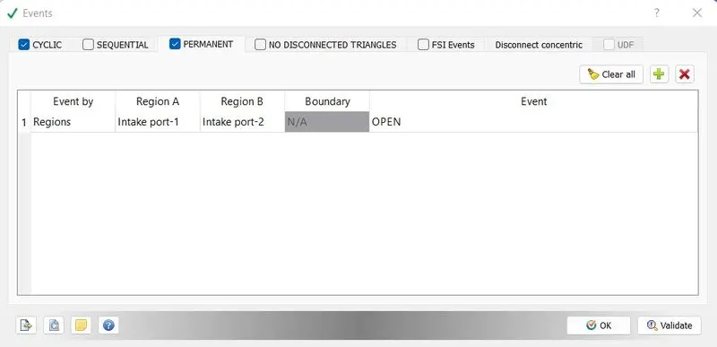
• A permanent event is setup between intake port-1 and intake port-2
• Once events are setup, base grid mesh size is specified and the files are exported to a folder and run in cygwin.
• The next important steps are setting up full hydro setup. For that, first we need to setup parcel simulation.
• Parcels are fuel droplets collections into the domain at the injector. Each parcel represents a group of identical spherical drops.
• At first, under liquids->Parcel select isooctane.
• 
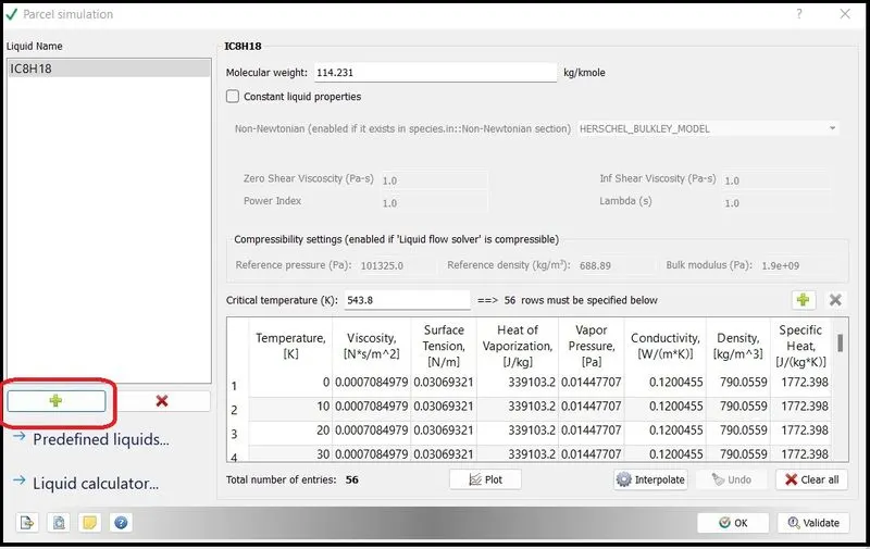
• To create a parcel,click on the add icon as shown above and you must be able to select isooctane from the list. Select it and click OK.
• 
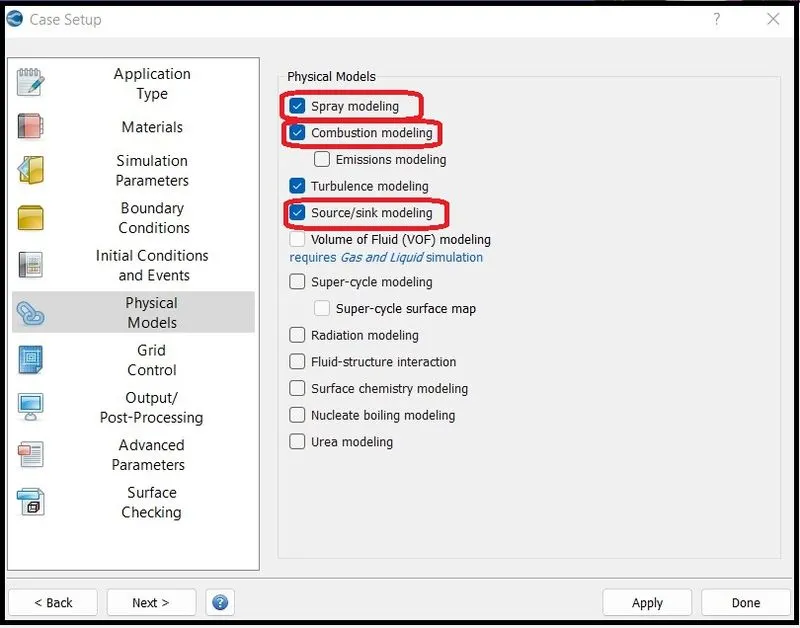
• Once parcel is setup, the next setup is to establish spray modeling, combustion modelling and source and sink modelling.
• At first, combustion modeling is setup as shown below:
• 
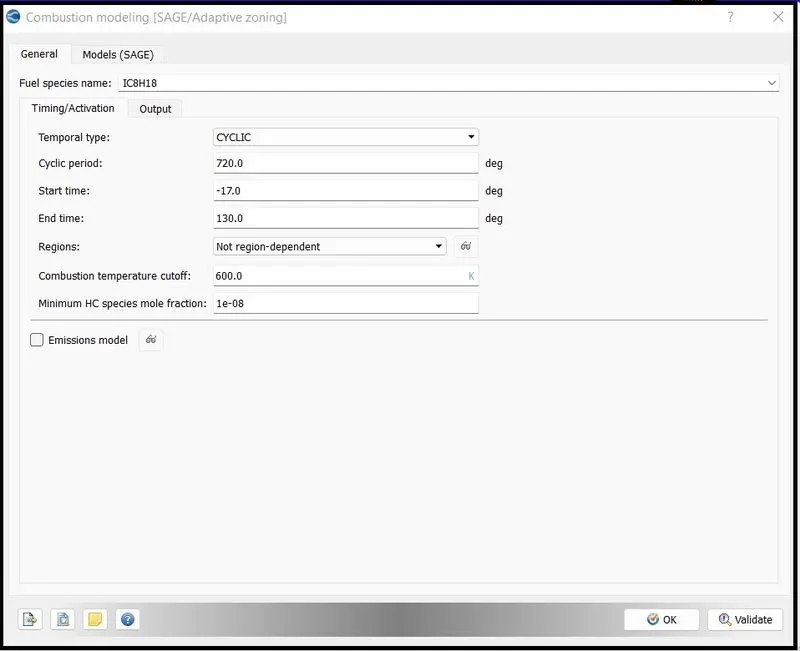
• Here, SAGE model is chosen for this case.
• SAGE detailed chemistry solver:The most predictive and accurate way to model combustion.Accurately model ignition and laminar flame propagation. SAGE detailed chemistry solver uses local conditions to calculate reaction rates based on the principles of chemical kinetics. This solver is fully coupled to the flow solver, but the chemistry and flow solvers parallelize independently of one another, which speeds up the simulation. With the appropriate mechanism, the SAGE solver can predict a wide range of cases (e.g., a variety of fuels [premixed, non-premixed, partially premixed, multiple fuels], emissions modelling, and unique phenomena such as end-gas auto-ignition). With its accuracy and robustness, CONVERGE can perform predictive modelling instead of merely confirming experimental results.
• 
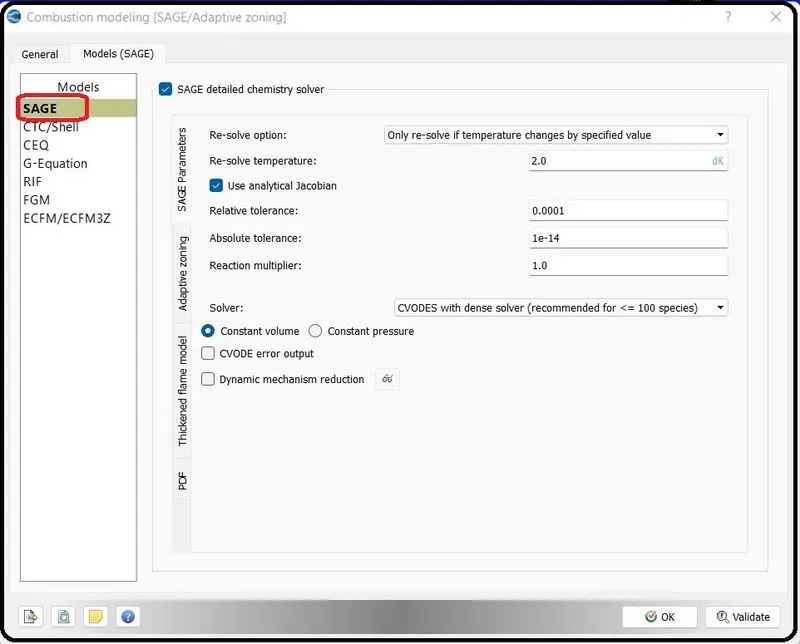
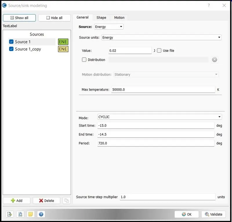
• Next, source and sink model is setup. This modeling is chosen so that the energy needed to be supplied by the spark plug can be specified. Note that the start times and end times are specified so that the energy is added only during combustion stroke and that too for a short duration of time.
• 
• Once that is done, the final step is to setup the spray modeling.
• This is important because we need to specify the time at which fuel needs to be injected and the type of dispersion that should be applied.
• 
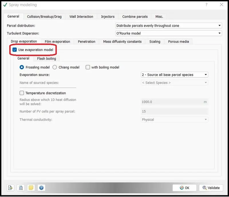
• The evaporation model is chosen. The evaporation source is chosen as 'Source all base parcel species'
• Go to collisions tab and choose the drag drop model as 'dynamic drag drop model'. This ensures that the drops will vapourise at a certain length called impingement length.
• 
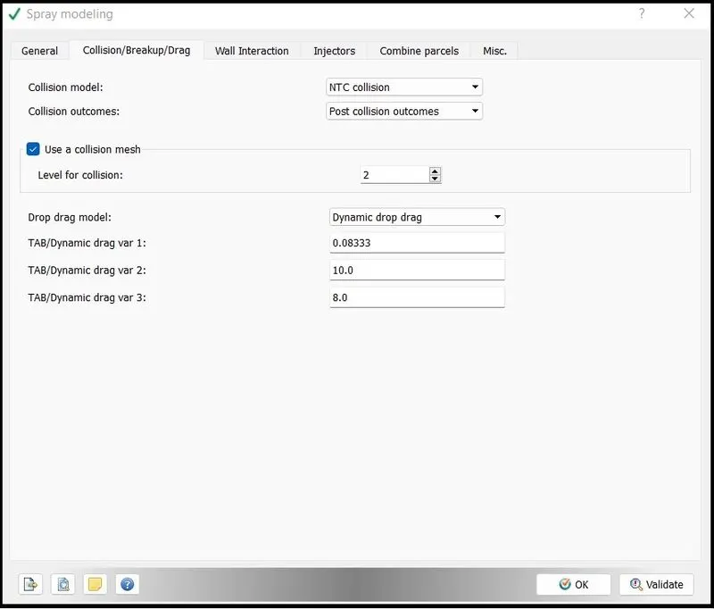
• Choose the collision model as NTC model.
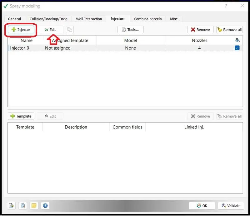
• Go to the injectors tab and click on add injector button. Once done, click on edit button to specify nozzle cone parameters of the spray as follows:
• 
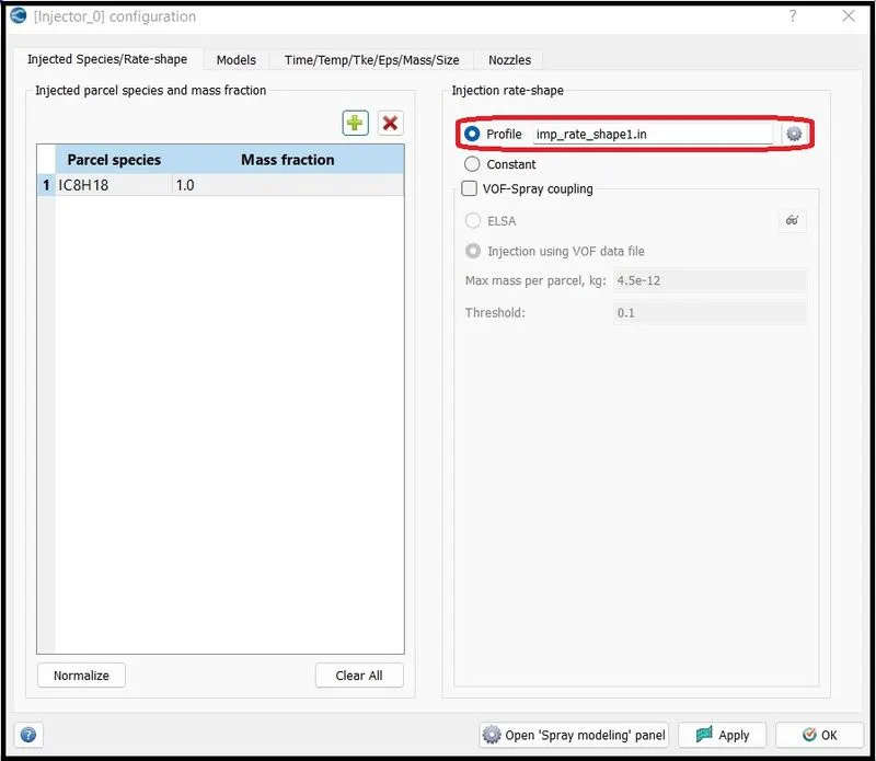
• At first, under injectors->Species tab click on add icon and click on the parcel species and enter the mass fraction as 1. Choose the profile by clicking on the setting icon and click ok.
• 
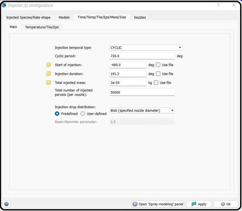
• Once done, click on the models tab. This is where we specify the start time and duration of fuel injection. Once done, the final step is to setup the nozzle cone parameters.
• 
• Go to nozzles tab and click on add nozzle as shown below.
• 
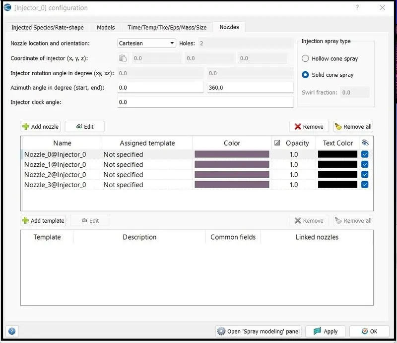
• A dialog box will appear in which we have to specify the dimensions of the nozzle as shown below:
• 
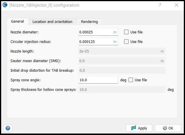
• The dimensions of all the four nozzles are specified below:

• Nozzle positions	Nozzle centre	Align vector
  Nozzle 0	(0.0823357,0.00100001 ,0.07019)	(-0.732501,0.210489 ,-0.647408)
  Nozzle 1	(0.0823357,-0.00099999 ,0.07019)	(-0.732501,-0.210489 ,-0.647408)
  Nozzle 2	(0.0823357,-0.0004 ,0.07019)	(-0.5,-0.2,-0.647408)
  Nozzle 3	(0.0823357,0.0003,0.07019)	(-0.5,0.2,-0.647408)

• Once all the nozzle positions are specified, that completes spray modeling setup

Fixed embedding:

Depending on the flow taking place, we may require that the flow at some region is more accurate and at some region is more approximate. This can be done by varying the mesh element sizes in the region. The embedding option in Converge CFD does this work of creating finer mesh at the mentioned location. The refinement is based on the scale and number of embed layers. If the base mesh created has cubic elements of size 'E' mm then the scale of 'n' means the elements in the refinement region will be of size `E/2^n` mm. This means that if the base mesh has elements of size 4 mm then elements of scale 1, 2, 3, 4, 5 will have elements of size 2, 1, 0.5, 0.25, 0.125 mm respectively. With each element scale, there is 8 times increase in total cell count. This happens because the elements are divided in size by 2 in all directions (X, Y, Z).

Fixed embedding is provided near valve angles as the space between valve angle and valve seat is very small and base grid with 0.004 m grid size will give inaccurate results.

Fixed embedding is provided to refine the specific areas and capture the combustion details and calculate them properly.

Cylindrical shape type embedding is provided on the cylinder to make them finer as compared to the base grid.

Adaptive Mesh Refinement:

The fixed embedding setting is preferred when the refinement is needed in the complete region or complete boundary area. When the refinement is to be done based on the solution of flow equations, the refinement technique is called AMR. The AMR monitors the solution and based on the curvature (second degree of rate of change) of a variable, the mesh is refined. There are two methods to use AMR: Sub-grid scale method and Value-based method. In the value-based method, the value of a solution is specified. If the value is more/less than specified, the mesh is refined. The Sub-grid method works in the following way:

For a scalar, the sub-grid field is defined as the difference between the actual field and the resolved field or

This sub-grid can also be represented as an infinite series, but since it's not possible to evaluate the entire series, only the first term in the series is used to approximate the scale of the subgrid.

A cell is embedded if the absolute value of the sub-grid field is above a user-specified value. Conversely, a cell is released (i.e., the embedding is removed) if the absolute value of the subgrid is below 1/5th of the user-specified value. That means if the user specifies a value of 2.5, the mesh program would calculate sub-grid of the cell, based on the term shown above and if it is larger than 2.5, the cell will be refined.

Regions and Events

In an actual engine, periodically the valves and ports are in contact with each other, which prevents flow between these parts of the engine. To control the flow while avoiding intersecting triangles, converge adds or removes virtual triangles(disconnect triangles) at user specified times called events.

In IC engines, we have ring triangles set up or removed at user specified times so as to simulate opening and closing of the valves.

Results and discussions

Pressure animation inside cylinder

Velocity animation inside cylinder

CO2 animation

The spray pattern in each case involve fuel entering the cylinder and getting compressed.

Compression ratio(r)

Compression ratio is defined as the the ratio of total volume of the engine divided by the clearance volume

`r=V_t/V_c`

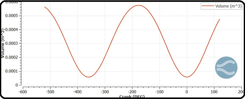
The above figure depicts the variation of volume as a function of crank angle. The crests and troughs depict the four stroke of the engine i.e during intake stroke, volume is large, during compression, volume is compressed and during power stroke, hot gases again expand and during exhaust stroke, the piston pushes the gas ot through the exhaust port and hence the volume decreases.

From the above figure, we can conclude that

r=`0.0005722/(5.7e-05)`=10.1

Combustion efficiency

Combustion efficiency is the amount of heat released during combustion inside engine over theoretical energy released by fuel during one complete cycle of the engine.

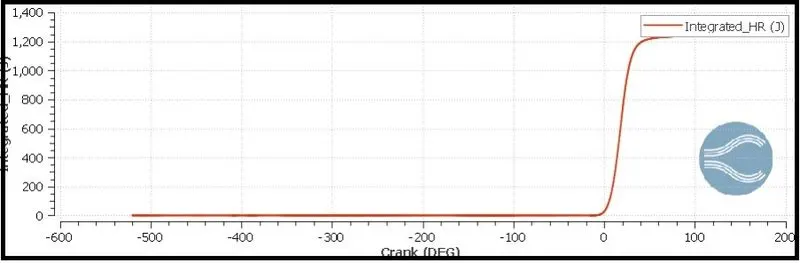
Note that for iso-octane, calorific value-44.4MJ/kg where M->mega

`Combustion efficiency=(Actual value)/(Calorific Value)`

`implieseta=1200/(44.4*10^6*3*10^-5)=0.92`

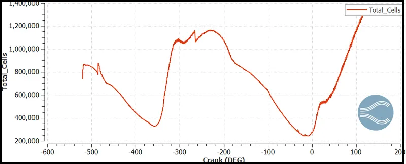
Total cell count

Need for wall heat transfer model

IC engines are developed continuously owing to their high power to weight ratio. In that case, optimizing any one aspect of the engine involves using theoretical models like spray model and combustion model which are described earlier, the better the model the better the accuracy of the results that are obtained.

To perform good prediction of engine heat transfer and wall temperature, models are required for accomplishing heat transfer from hot gases to engine parts, heat transfer inside each engine part, and also heat transfer to coolant and lubricating oil. This paper presents an overview of engine heat transfer and wall temperature modelling, with the main purpose to aid engine thermodynamic modelling and offer more accurate predictions of engine performance, consumption and emission parameters. The most important are three engine heat transfer approaches: gas to the wall, wall to wall and wall to liquid heat transfer models. To obtain a good prediction of wall temperature, those three approaches must be coupled, which may imply convection-conduction-convection problems, although, for some applications in diesel engines, radiation problems must be considered.

Therefore, using only a CFD approach wont' help in capturing the accurate details at the walls. Instead a CHT analysis will enable us to calculate wall heat transfer coefficients.

Engine performance calculator

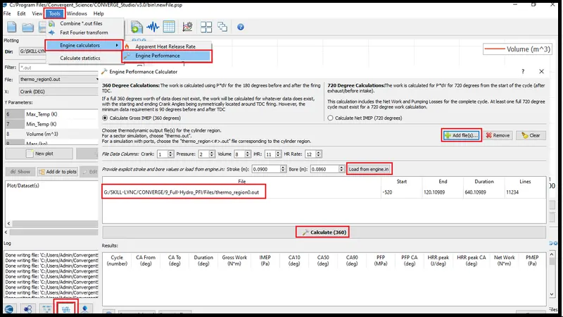
It is used to calculate and analyse physical data and get useful results from the data.

To use this tool, go to line plotting tool available at the extreme left end of the studio page.

Go to tools->engine calculator and select engine performance and add thermo_region0.out and engine.in files respectively.

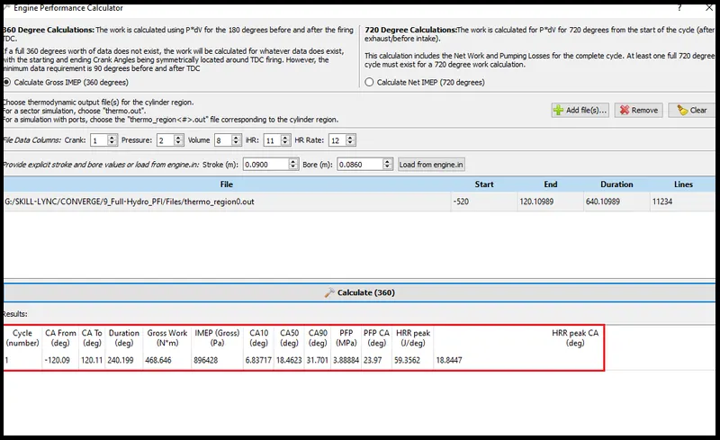
CA->crank angle.

Significance of CA

The CA refers to Crank Angle followed by its position in a degree at 10%, 50% & 90%. These angles are captured to store the data such as heat release, combustion data. The significance of it is that CA10 is used to determine the start of ignition, CA50 determines the end of premixed combustion and CA10-90 determines combustion duration and at CA90 the burning of unburnt fuel is done by the propagating flame. If CA90 value is large, the crank angles are taken increases and the exhaust stroke tends to push the premature combustion products. This data is used to compare the simulation data from experimental results or simulation data from previous results at specified percentages. Parameters like the accuracy of pegging, encoder phasing, trapped mass estimate, Volume estimate, heat generation etc. Combustion phasing angles of heat release are determined by integrating the AHRR.

CA 10(deg) = 6.83717 degree

CA 50(deg) = 18.4623 degree

CA 90(deg) = 31.701 degree

Power is the rate of work done i.e, the amount of work done per unit time.

WKT engine rpm-3000

Therefore, rps-50

dps(degrees per second)=360*50=18000

Time per degree=`1/(dps`=`5.555e-5`

For one cycle, time taken=240*1/dps=0.11331s

`implies Power=(Work)/(time)`=35.12kW

Since Work and Torque has the same unit (N-m) , it doesn't mean value for Torque and Work will be the same. Both are different quantities and has totally different meaning. So the value for work got from the engine performance calculator is not the value for the torque. Note that while work is the force exerted to cause a motion, torque is the angular version of force.

It is calculated from the formula:

`P=(2piNT)/60`, where T->Torque

`impliesT=(60P)/(2piN)=111 Nm`

Note that torque and rpm are inversely related. A large torque implies smaller rpm.

Spray droplet variation

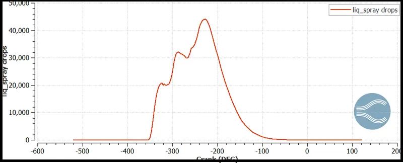
In the above plot, the peak value shows around 44000 parcels and further parcels actually start to drop this is because of vaporization and combustion takes place. Towards the end, we can see zero parcels that means there is not much fuel left which indicates there won't be a lot of unburnt HC.

Total no of droplets

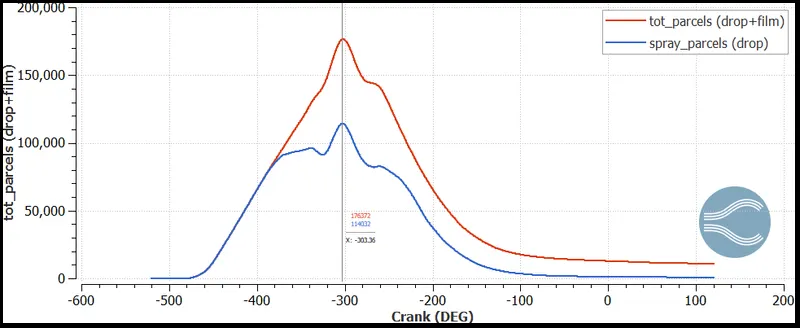
The parcels increased as injection started. The parcels started collecting in films on the cylinder wall when the intake valves were open. This is because when the intake valves were fully open, the fuel spray was directly hitting the cylinder wall.

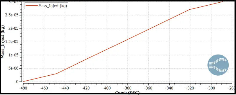
This is variation of mass flow rate of fuel injected, which matches closely with our theoretical value of 3e-05 kg.

Thus the full hydro simulation of PortFuelInjection engine is conducted and the values are studied.