Week 8: Literature review - RANS derivation and analysis

Literature review - RANS derivation and analysis

In this challenge, we shall derive reynolds averaged navier stokes equation and come up with the expression for reynolds stress. Also we shall see what is reynolds stress, and what is turbulent viscosity and how it is different from molecular viscosity.

Theory

All flows encountered in engineering practice, simple ones, such as twodimensional jets, wakes, pipe flows and flat plate boundary layers, and more complicated three-dimensional ones, become unstable above a certain Reynolds number (UL/ν where U and L are characteristic velocity and length scales of the mean flow and ν is the kinematic viscosity). At low Reynolds numbers flows are laminar. At higher Reynolds numbers flows are observed to become turbulent. A chaotic and random state of motion develops in which the velocity and pressure change continuously with time within substantial regions of flow.

Lets take a brief look at the main characteristics of turbulent flows. The Reynolds number of a flow gives a measure of the relative importance of inertia forces (associated with convective effects) and viscous forces. In experiments on fluid systems it is observed that at values below the so called critical Reynolds number `underset(crit)(Re)` the flow is smooth and adjacent layers of fluid slide past each other in an orderly fashion. If the applied boundary
conditions do not change with time the flow is steady. This regime is called laminar flow.

At values of the Reynolds number above `underset(crit)(Re)`a complicated series of events takes place which eventually leads to a radical change of the flow character. In the final state the flow behaviour is random and chaotic. The motion becomes intrinsically unsteady even with constant imposed boundary conditions. The velocity and all other flow properties vary in a random and chaotic way. This regime is called turbulent flow.

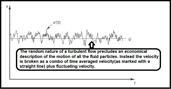
Even in flows where the mean velocities and pressures vary in only one or two space dimensions, turbulent fluctuations always have a threedimensional spatial character.

Derivation of the equations

Let us consider a single point measurement in a turbulent flow.The Reynolds decomposition defines flow property ϕ at this point as the sum of a steady mean component Φ and a time varying fluctuating component ϕ′(t) with zero mean value

Hence ϕ (t) = Φ +ϕ′(t).

The mean Φ of flow property ϕ is defined as follows:

`Φ = (1/(Deltat))int_0^(Deltat)ϕ (t) dt`

The time average of the fluctuations ϕ ′ is, by definition, zero.

`barϕ′(1/(Deltat))int_0^(Deltat)ϕ ′(t) dt ≡ 0`

From now on we shall not write down the time-dependence of ϕ and ϕ ′ explicitly, so we write ϕ = Φ +ϕ ′.

Reynolds-averaged Navier Stokes equations for incompressible flow

We begin by summarising the rules which govern time averages of fluctuating properties ϕ = Φ +ϕ′ and ψ = Ψ +ψ′ and their summation, derivatives and integrals:

`bar(phi')=bar(psi')=0`

`bar(phi)=phi;bar(delphi)/(dels)=(delphi)/(dels);int(bar(phi)ds)=int(phids)`

To start with we consider the instantaneous continuity and Navier–Stokes equations in a Cartesian co-ordinate system so that the velocity vector V has x-component u, y-component v and z-component w:

`grad.V=0`

`(delu)/(delt)+grad.(uV)=(-1/rho)*(delP)/(delx) +nugrad.grad(u)`

`(delv)/(delt)+grad.(vV)=(-1/rho)*(delP)/(dely) +nugrad.grad(v)`

`(delu)/(delt)+grad.(wV)=(-1/rho)*(delP)/(delz) +nugrad.grad(z)`

This system of equations governs every turbulent flow, but we investigate the effects of fluctuations on the mean flow using the Reynolds decomposition in the above four equations and replace the flow variables V (hence
also u, v and w) and p by the sum of a mean and fluctuating component.

`v = V + v′; u = U + u′ ;v = V+ v′ ;w = W + w′; p = P + p′`

This yields the continuity equation for the mean flow:

`grad.u=0`

`bar(delu)/(delt)=(delU)/(delt)` `bar(grad.(uV))=grad.(uU)+grad.bar(u'v')`

and so on...

Substitution of these results gives the time average x momentum equation

`(delu)/(delt)+grad.(uV)+grad.(bar(u'v'))=(-1/rho)*(delP)/(delx) + nu*grad.gradu`

`(delv)/(delt)+grad.(vV)+grad.(bar(v'v'))=(-1/rho)*(delP)/(dely) + nu*grad.gradv`

`(delW)/(delt)+grad.(wV)+grad.(bar(w'v'))=(-1/rho)*(delP)/(delz) + nu*grad.gradw`

Note that these three equations are similar to the NS equations mentioned at the beginning of this challenge.

We have also introduced new terms in the resulting time-average momentum equations. The terms involve products of fluctuating velocities and are associated with convective momentum transfer due to turbulent
eddies. The above equations are rewritten as

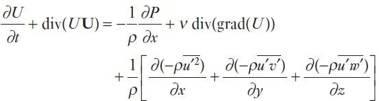
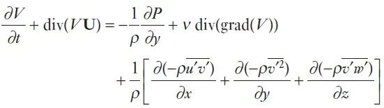
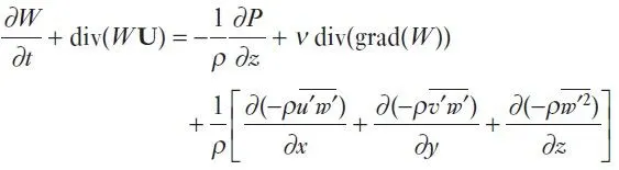
The extra stress terms have been written out in longhand to clarify their structure. They result from six additional stresses:

three normal stresses `underset(x x)(tau)=-rho*bar(u'^2);underset(y y)(tau)=-rho*bar(v'^2);underset(z z)(tau)=-rho*bar(w'^2)`

and three shear stresses:`underset(x y)(tau)=-rho*bar(u'v')=underset(y x)(tau);underset(y z)(tau)=-rho*bar(v'w')=underset(z y)(tau);underset(z x)(tau)=-rho*bar(w'u')=underset(x z)(tau)`

These extra turbulent stresses are called the Reynolds stresses. The normal stresses involve the respective variances of the x-, y- and z-velocity fluctuations. They are always non-zero because they contain squared velocity fluctuations. The shear stresses contain second moments associated with correlations between different velocity components. Reynolds stress is a component of stress tensor in fluid which is obtained by averaging operation over the Navier Stokes equation used to account for turbulent fluctuation in the fluid.

Turbulent Viscosity is a function of fluctuations in velocity and is influenced by the randomness of flow. It is non-linear and difficult to estimate. It depends upon flow regimes and is not a property. It is dominant in turbulent flow regimes with high Reynolds numbers.

Molecular Viscosity is due to the internal resistance amongst different molecular layers. This viscosity offers resistance to any deformation under the application of an external force and is an independent property.

This equation set is called Reynolds averaged navier stokes equation

Turbulence causes the appearance in the flow of eddies with a wide range of length and time scales that interact in a dynamically complex way. Given the importance of the avoidance or promotion of turbulence in engineering
applications, it is no surprise that a substantial amount of research effort is dedicated to the development of numerical methods to capture the important effects due to turbulence. The methods can be grouped into the following three categories:

• Turbulence models for Reynolds-averaged Navier–Stokes (RANS) equations:The Navier–Stokes equations are time averaged (or ensemble averaged in flows with time-dependent boundary conditions). Extra terms appear in the time-averaged (or Reynoldsaveraged) flow equations due to the interactions between various turbulent fluctuations. These extra terms are modelled with classical turbulence models: among the best known ones are the k–ε model and the Reynolds stress model. The computing resources required for reasonably accurate flow computations are modest, so this approach has been the mainstay of engineering flow calculations over the last three decades.
• Large eddy simulation: this is an intermediate form of turbulence calculations which tracks the behaviour of the larger eddies. The method involves space filtering of the unsteady Navier–Stokes equations prior to the computations, which passes the larger eddies and rejects the smaller eddies. The effects on the resolved flow (mean flow plus large eddies) due to the smallest, unresolved eddies are included by means of a so-called sub-grid scale model. Unsteady flow equations must be solved, so the demands on computing resources in terms of storage and volume of calculations are large, but (at the time of writing) this technique is starting to address CFD problems with complex geometry.
• Direct numerical simulation (DNS): these simulations compute the mean flow and all turbulent velocity fluctuations. The unsteady Navier–Stokes equations are solved on spatial grids that are sufficiently fine that they can resolve the Kolmogorov length scales at which energy dissipation takes place and with time steps sufficiently small to resolve the period of the fastest fluctuations. These calculations are highly costly in terms of computing resources, so the method is not used for industrial flow computations.

Use of RANS model

For most engineering purposes it is unnecessary to resolve the details of the turbulent fluctuations. CFD users are almost always satisfied with information about the time-averaged properties of the flow (e.g. mean velocities,
mean pressures, mean stresses etc.). Therefore, the vast majority of turbulent flow computations has been and for the foreseeable future will continue to be carried out with procedures based on the Reynolds-averaged Navier–Stokes (RANS) equations.

Note:

In viscous sublayer, flow is laminar. Therefore, inertial terms are negligible and pressure drop is negligible,which gives

`u*bar(delu)/(dely) -rho/(Deltat)int_0^(Deltat)u'v'dt=constant`

Outside viscous sublayer, turbulent viscosity dominates.

`implies`shear stress =`rho/(Deltat)int_0^(Deltat)u'v'dt`

Let `1/(Deltat)int_0^(Deltat)u'v'dt =(u^**)^2`

Then `tau=rho*(u^**)^2`

`impliesu^**=sqrt(tau/rho)`

We define a non dimensional velocity `u^+=baru/u^**``impliesu^+=baru*sqrt(rho/tau)`

We also a non dimensional distance `y^+=y/(L_c) =y/(nu/u^**)=y*u^**/nu`

When `y^+` is very small, we are in the viscous sublayer.

So in viscous sublayer,`y^+=u^+`

whereas in turbulent region, `u^+=(1/k)ln(y^+)+C`

Thus the RANS equation is derived and the importance of y+ and u+ are mentioned as well.