Week 11 - Simulation of Flow through a pipe in OpenFoam
Challenge
In this challenge, an axi-symmetric flow is simulated by applying the wedge boundary condition. The flow is laminar and flows through a constant cross-section pipe at an inlet Reynold's number of 2100. The results are then validated with the Hagen- Poiseuille's equations for the fully developed flow.
Generally, viscous flows are classified into laminar flow and turbulent flow. A laminar flow is one in which the flow is streamlined and the fluid particles move in an orderly manner. A turbulent flow is one in which the streamlines move in a chaotic fashion. A transition region is one in which the flow changes from laminar to turbulent.
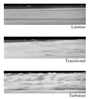
The given case corresponds to an internal flow. In an internal flow, if the reynolds number crosses 2400, the flow is said to be turbulent.
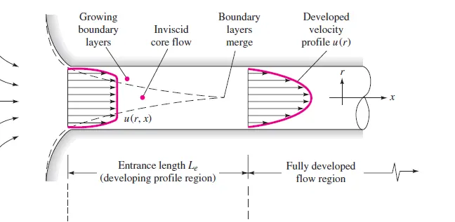
The above example corresponds to a pipe flow commonly termed as hagen-poiseuille flow. Since the pipe flow is a viscous flow, at the entry section of the pipe, boundary layer begins to develop from both the walls of the cross-section. There is a distance along the length of the pipe at which the boundary layer fully develops.It is called as the entrance length. After the entrance length, the flow becomes fully developed.
Since the reynolds' no is given as 2100, and assuming that the pipe diameter(D) be 1 cm or 0.01 m,
`Re=(rho.V.D)/mu` =`(V*D)/nu` where `mu`->dynamic viscosity `nu`->kinematic viscosity
The results of Hagen-Poiseuille flow are listed below:
`underset(e)(L)=0.06*Re*D` where `underset(e)(L)`->hydrodynamic entry length
`underset(max)(V)=2*underset(avg)(V)`
From reynolds number calculation, we get V=0.21 m/s
Since the flow is laminar, `underset(e)(L)`=1.26m
Therefore, assume the entire length of the pipe as 2.52 m.
The pressure drop over a pipe of length L is`DeltaP=(32*underset(avg)(U)*mu*L)/D^2`
The max shear stress is `underset(max)(tau)=(2*mu*underset(max)(V)*R)/r^2`
The shear stress variation is given as`tau=mu*(delV)/(delr)`
Geometry and Meshing
Since the simulation of a pipe takes a lot of time, lts simulate a portion of the pipe. A wedge is a portion of the pipe, as shown below
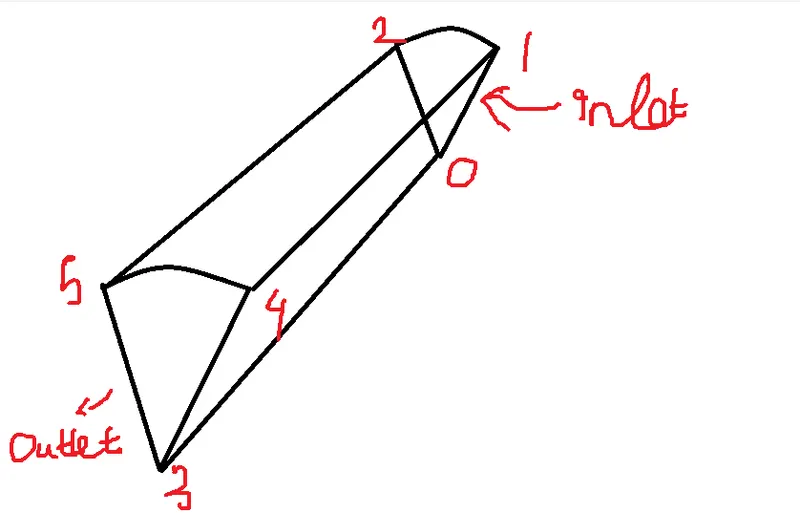
Here, the wedge angle is assumed to be small(<`5 ^o`). The blocks are considered as a ccombination of the wedge face and arcs and lines. To generate the geometry in blockMeshDict file, the challenge is to automate this process so that an input is fed to a computer program, which then takes into MATLAB and parses the file. A program is written in matlab to achieve this, and file parsing is performed.
The coordinates considered are:
inlet (0 1 2 0)
outlet (3 5 4 3)
wall (1 4 5 2)
axis (0 3 3 0)
wedgefront (0 3 4 1)
wedgeback (0 2 5 3)
File Parsing in MATLAB
File parsing is the process by which information can be read from a particular file and how that information can be used in a computer program. In this challenge, the blockmesh file is parsed by writing a code in matlab and the file is shared with Linux platform in the OpenFOAM run folder. After that, the process is continued and the initial values are
f1=fopen('blockMeshDict.txt','w');
l1='/*-----------------------------*- C++ -*---------------------------------*';
l2='      =========                   |';
l3='      \      /   F  ield         |  OpenFOAM: The Open Source CFD toolbox';
l4='       \    /    O  peration     |  Website:  https://openfoam.org/';
l5='        \  /     A  nd           |  Version:  9';
l6='         \/      M  anipulation  |  ';
l7='*-----------------------------------------------------------------------*/';
l8='FoamFile';
l9='{ ';
l10='    format    ascii;';
l11='    class     dictionary;';
l12='    object    blockMeshDict;';
l13='} ';
l14='// * * * * * * * * * * * * * * * * * * * * * * * * * * * * * * * * * * * *//';
l15='convertToMeters 1;';
l16=' ';
l17='vertices';
l18='(';
l19=');';
fprintf(f1,'%sn',l1);
fprintf(f1,'%sn',l2);
fprintf(f1,'%sn',l3);
fprintf(f1,'%sn',l4);
fprintf(f1,'%sn',l5);
fprintf(f1,'%sn',l6);
fprintf(f1,'%sn',l7);
fprintf(f1,'%sn',l8);
fprintf(f1,'%sn',l9);
fprintf(f1,'%sn',l10);
fprintf(f1,'%sn',l11);
fprintf(f1,'%sn',l12);
fprintf(f1,'%sn',l13);
fprintf(f1,'%sn',l14);
fprintf(f1,'%sn',l15);
fprintf(f1,'%sn',l16);
fprintf(f1,'%sn',l17);
fprintf(f1,'%sn',l18);
v=0.21;        %velocity of the flow
Re=2100;       %reynolds number of the flow
D=0.01;        %diameter in m
r=D/2;         %radius in m
L_h=0.06*Re*D; %entry length of the pipe
L=L_h+0.7;       %full length
v_max=2*v;     %max velocity
theta=4;
%coordinates
c0=[0 0 0];    %zero coordinate
c1=[0 r*cosd(theta/2) r*sind(theta/2)];
c2=[0 r*cosd(theta/2) -r*sind(theta/2)];
c3=[L 0 0];
c4=[L r*cosd(theta/2) r*sind(theta/2)];
c5=[L r*cosd(theta/2) -r*sind(theta/2)];
d1=[300 50 1];  %number of divisions
gf=.2;            %grading factor
arc1=[0 r 0];    %arc passing through the point
arc2=[L r 0];    %arc passing through the point
fprintf(f1,'t (%.3f %.3f %.3f) n',c0);
fprintf(f1,'t (%.3f %.3f %.7f) n',c1);
fprintf(f1,'t (%.3f %.3f %.7f) n',c2);
fprintf(f1,'t (%.3f %.3f %.3f) n',c3);
fprintf(f1,'t (%.3f %.3f %.7f) n',c4);
fprintf(f1,'t (%.3f %.3f %.7f) n',c5);
fprintf(f1,'%s n',l19);
fprintf(f1,'%s','blocks');
fprintf(f1,'n%s','(');
fprintf(f1,'t %s (%d %d %d) %s (1 %d 1)n','hex (0 3 5 2 0 3 4 1)',d1,'simpleGrading',gf);
fprintf(f1,'n%s',');');
fprintf(f1,'n%sn%s','edges','(');
fprintf(f1,'nt%st(%.3f %.3f %.3f)','arc 1 2',arc1);
fprintf(f1,'nt%st(%.3f %.3f %.3f)','arc 4 5',arc2);
fprintf(f1,'n%s',');');
fprintf(f1,'n%sn%s','boundary','(');
fprintf(f1,'nt%snt%sntt%s','inlet','{','type patch;');
fprintf(f1,'ntt%sntt%s','faces','(');
fprintf(f1,'n%25sntt%snt%s','(0 1 2 0)',');','}');
fprintf(f1,'nt%snt%sntt%sntt%sntt%s','outlet','{','type patch;','faces','(');
fprintf(f1,'n%25sntt%snt%s','(3 5 4 3)',');','}');
fprintf(f1,'nt%snt%sntt%sntt%sntt%s','wall','{','type wall;','faces','(');
fprintf(f1,'n%25sntt%snt%s','(1 4 5 2)',');','}');
fprintf(f1,'nt%snt%sntt%sntt%sntt%s','axis','{','type empty;','faces','(');
fprintf(f1,'n%25sntt%snt%s','(0 3 3 0)',');','}');
fprintf(f1,'nt%snt%sntt%sn%13sn%9s','wedgeFront','{','type wedge;','faces','(');
fprintf(f1,'n%25sntt%snt%s','(0 3 4 1)',');','}');
fprintf(f1,'nt%snt%sntt%sn%13sn%9s','wedgeBack','{','type wedge;','faces','(');
fprintf(f1,'n%25sntt%snt%sn%s','(0 2 5 3)',');','}',');');
fprintf(f1,'n%sn%sn%s','mergePatchPairs','(',');');
Generated Blockmesh
/*--------------------------------*- C++ -*----------------------------------*
  =========                 |
  \      /  F ield         | OpenFOAM: The Open Source CFD Toolbox
   \    /   O peration     | Website:  https://openfoam.org
    \  /    A nd           | Version:  9
     \/     M anipulation  |
*---------------------------------------------------------------------------*/
FoamFile
{
    format      ascii;
    class       dictionary;
    object      blockMeshDict;
}
// * * * * * * * * * * * * * * * * * * * * * * * * * * * * * * * * * * * * * //

//convertToMeters 1;

vertices
(
	 (0.000 0.000 0.000)
	 (0.000 0.00499 0.0001745)
	 (0.000 0.00499 -0.0001745)
	 (1.960 0.000 0.000)
	 (1.960 0.00499 0.0001745)
	 (1.960 0.00499 -0.0001745)
);
blocks
(	 hex (0 3 5 2 0 3 4 1) (300 50 1) simpleGrading (1 0.1 1)

);
edges
(
	arc 1 2	(0.000 0.005 0.000)
	arc 4 5	(1.960 0.005 0.000)
);
boundary
(
	inlet
	{
		type patch;
		faces
		(
                (0 1 2 0)
		);
	}
	outlet
	{
		type patch;
		faces
		(
                (3 5 4 3)
		);
	}
	wall
	{
		type wall;
		faces
		(
                (1 4 5 2)
		);
	}
	axis
	{
		type empty;
		faces
		(
		(0 3 3 0)
		);
	}
	wedgeFront
	{
		type wedge;
        faces
        (
                (0 3 4 1)
		);
	}
	wedgeBack
	{
		type wedge;
        faces
        (
                (0 2 5 3)
		);
	}
);
mergePatchPairs
(
);

// ************************************************************************* //

// ************************************************************************* //
Initial values:
The kinematic pressure is initialized.
Pressure
/*--------------------------------*- C++ -*----------------------------------*
  =========                 |
  \      /  F ield         | OpenFOAM: The Open Source CFD Toolbox
   \    /   O peration     | Website:  https://openfoam.org
    \  /    A nd           | Version:  9
     \/     M anipulation  |
*---------------------------------------------------------------------------*/
FoamFile
{
    format      ascii;
    class       volScalarField;
    object      p;
}
// * * * * * * * * * * * * * * * * * * * * * * * * * * * * * * * * * * * * * //

dimensions      [0 2 -2 0 0 0 0];

internalField   uniform 0;

boundaryField
{
    inlet
    {
        type            zeroGradient;
    }

    outlet
    {
        type            fixedValue;
	value		uniform 0.1317;
    }

    wall
    {
        type            zeroGradient;
    }
    wedgeFront
    {
        type		wedge;
    }
    wedgeBack
    {
        type		wedge;
    }
    axis
    {
    	type		empty;
    }

}

// ************************************************************************* //
Velocity
The inlet velocity calculated from the reynolds number is used as the inlet condition.
/*--------------------------------*- C++ -*----------------------------------*
  =========                 |
  \      /  F ield         | OpenFOAM: The Open Source CFD Toolbox
   \    /   O peration     | Website:  https://openfoam.org
    \  /    A nd           | Version:  9
     \/     M anipulation  |
*---------------------------------------------------------------------------*/
FoamFile
{
    format      ascii;
    class       volVectorField;
    object      U;
}
// * * * * * * * * * * * * * * * * * * * * * * * * * * * * * * * * * * * * * //

dimensions      [0 1 -1 0 0 0 0];

internalField   uniform (1 0 0);

boundaryField
{
    inlet
    {
        type            fixedValue;
        value           uniform (0.21 0 0);
    }

    outlet
    {
        type            zeroGradient;
    }

    wall
    {
        type            noSlip;
        value		uniform (0 0 0);
    }
    wedgeFront
    {
    	type		wedge;
    }
    wedgeBack
    {
    	type		wedge;
    }
    axis
    {
    	type		empty;
    }
}

// ************************************************************************* //
ControlDictionary:
The value of timestep interval is 0.01s. The solution will run for a period of 20 timesteps.
/*--------------------------------*- C++ -*----------------------------------*
  =========                 |
  \      /  F ield         | OpenFOAM: The Open Source CFD Toolbox
   \    /   O peration     | Website:  https://openfoam.org
    \  /    A nd           | Version:  9
     \/     M anipulation  |
*---------------------------------------------------------------------------*/
FoamFile
{
    format      ascii;
    class       dictionary;
    location    "system";
    object      controlDict;
}
// * * * * * * * * * * * * * * * * * * * * * * * * * * * * * * * * * * * * * //

application     icoFoam;

startFrom       startTime;

startTime       0;

stopAt          endTime;

endTime         20;

deltaT          1e-2;

writeControl    timeStep;

writeInterval   200;

purgeWrite      2;

writeFormat     ascii;

writePrecision  6;

writeCompression off;

timeFormat      general;

timePrecision   6;

runTimeModifiable true;


// ************************************************************************* //
Transport Properties
/*--------------------------------*- C++ -*----------------------------------*
  =========                 |
  \      /  F ield         | OpenFOAM: The Open Source CFD Toolbox
   \    /   O peration     | Website:  https://openfoam.org
    \  /    A nd           | Version:  9
     \/     M anipulation  |
*---------------------------------------------------------------------------*/
FoamFile
{
    format      ascii;
    class       dictionary;
    location    "constant";
    object      transportProperties;
}
// * * * * * * * * * * * * * * * * * * * * * * * * * * * * * * * * * * * * * //

nu              [0 2 -1 0 0 0 0] 1e-06;


// ************************************************************************* //
IcoFoam solver is used in this case. icoFOAM solver is used in a transient state for incompressible, laminar flow of fluids.
Once the solver finishes running, the contours are obtained and postprocessing is performed.
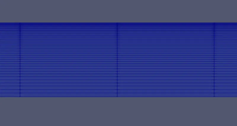
MESHING
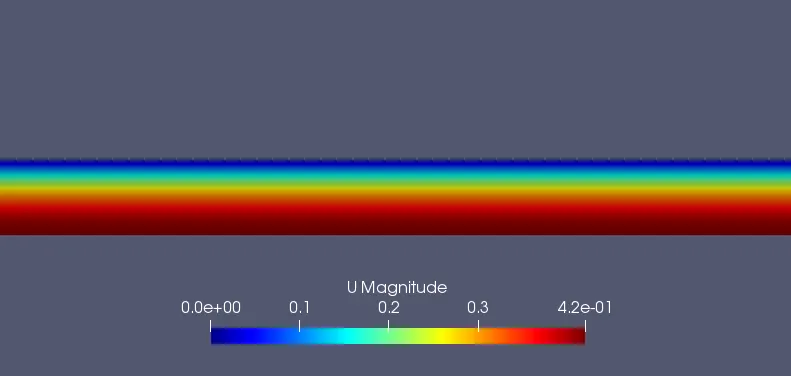
VELOCITY
Post-Processing in MATLAB
This stage involves comparing computational data with analytical data and drawing suitable inferences. For this case, the post processing is carried out in matlab. To do a comparison study between computational data and analytical data, we compare max velocity and shear stress values obtained in the calculation. A program is written in which the values(values of velocity and Pressure) that are obtained from Paraview are stored in an excel file and are read by matlab file. We have considered three cases- when length of the pipes are 0.2,0.5 and 1.3 m respectively.
The values are imported from the excel file into MATLAB and then stored inside variables. Analytical formulae are used to calculate analytical values.
%post processing of simulation of pipeflow in openfoam
data1=xlsread('x=1.2_0.5_0.2.xlsx','x=1.3','A1:B1002');      %1 corresponds to x=1.3
data2=xlsread('x=1.2_0.5_0.2.xlsx','x=0.5','A1:B1002');      %2 corresponds to x=0.5
data3=xlsread('x=1.2_0.5_0.2.xlsx','x=0.2','A1:B1002');      %3 corresponds to x=0.2
data4=xlsread('x=1.2_0.5_0.2.xlsx','Pressure variation','A1:B1002');
data5=xlsread('x=1.2_0.5_0.2.xlsx','Velocity variation','A1:B1002');
point1=data1(:,1);
velocity1=data1(:,2);
point2=data2(:,1);
velocity2=data2(:,2);
point3=data3(:,1);
velocity3=data3(:,2);
point4=data4(:,1);
pres=data4(:,2);
vel=data5(:,2);
%to calculate theoretical velocity distribution u=-(1/4mu)*(dp/dx)*(R^2-r^2)
mu=1e-03;
R=0.005;
r=linspace(0,0.005,1001);
dr=r(2)-r(1);
delp_dx=67.2;
vel_analyt=(1/(4*mu)).*(delp_dx).*(R^2-r.^2);
%to calculate analytical shear stress distribution
for i=2:length(vel_analyt)
    tau_analyt(i)=mu.*(vel_analyt(i)-vel_analyt(i-1))./dr;
end
%to calculate computed shear stress distribution
for i=2:length(velocity1)
    tau_computed(i)=mu.*(velocity1(i)-velocity1(i-1))./dr;
end
figure(1)
axis([0 0.5 0 0.005]);
plot(velocity1,point1,'r','linewidth',3);
hold on
plot(velocity2,point2,'b','linewidth',3);
hold on
plot(velocity3,point3,'g','linewidth',3);
hold on
plot(vel_analyt,r,'c','linewidth',3);
xlabel('Velocity');
ylabel('Radial distance');
legend('x=1.3','x=0.5','x=0.2','theoretical value');
figure(2)
plot(tau_analyt,point1,'r','linewidth',3);
hold on
plot(tau_computed,point1,'g','linewidth',3);
hold on
line([0 0],[0 R],'linewidth',3);
legend('theoretical shear stress variation','computed shear stress variation');
xlabel('Shear stress variation');
ylabel('Radial distance');
figure(3)
plot(point4,vel,'r','linewidth',3);
xlabel('length of the pipe');
ylabel('velocity in the pipe');
legend('Velocity variation');
figure(4)
plot(point4,pres,'g','linewidth',3);
xlabel('length of the pipe');
ylabel('pressure along the pipe');
legend('pressure variation');
RESULTS AND DISCUSSIONS:
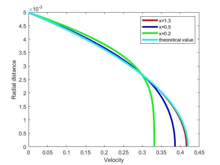
The above shows variation of velocity along the radius of the pipe from the axis to the wall. The above curve provides a comparison of the different velocity profiles at different sections along the length of the pipe. The analytical value matches with the computed value at a section length of 1.3 metre. The analytical values and the computed values are closely agreeing for the fully developed velocity profile.
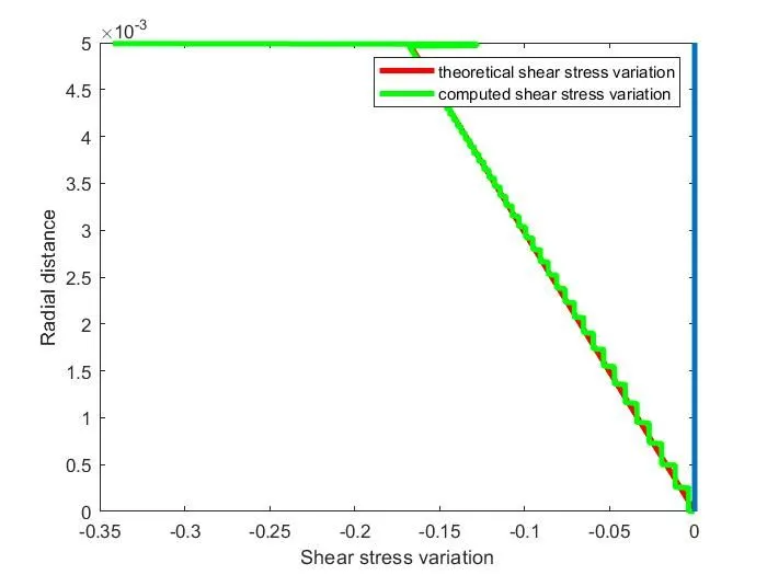
The analytical shear stress and computed shear stress are compared along the radial distance of the pipe. The step nature of the computed value of shear stress is because it is assumed that they obey first order backward differencing scheme. The graph shows that shear stress is max at the wall(where radius is 0.005 m) and minimum at the axis(where x=0). Since shear stress acts in an opposite direction to that of velocity, the values are in negative.
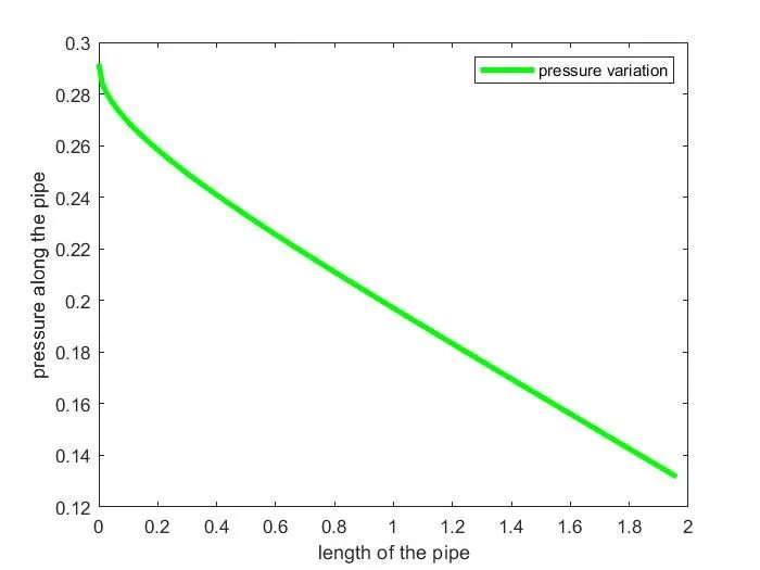
The kinematic pressure variation along the length of the pipe is shown in the plot above. Initially, the plot becomes smooth and curvy but after some distance, the slope becomes linear(i.e.`(delp)/(delx)=c`.
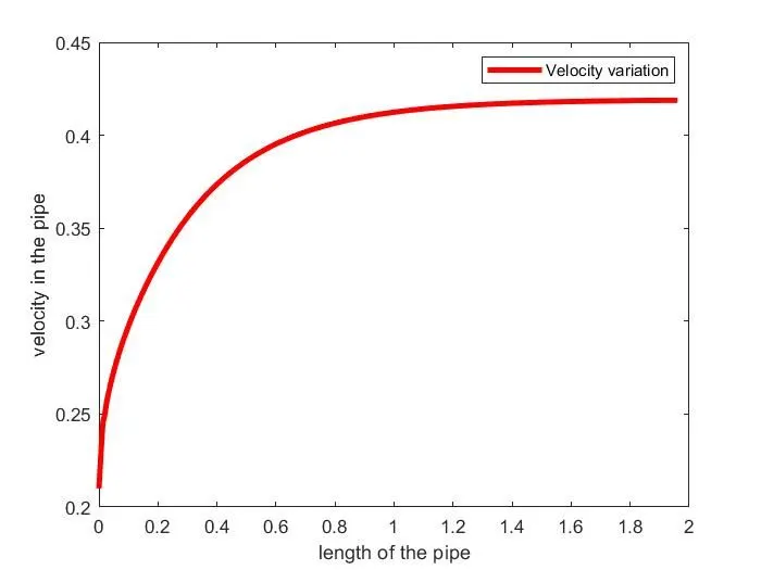
The variation of velocity along the length of the pipe is plotted above. The above variation can be explained as follows: Because at the inlet of the pipe, boundary layer develops along the wall and as a result, the flow gradually shows acceleration until a length called hydrodynamic entry length, beyond which the velocity becomes constant in a laminar flow. Until x=1.3 metre, we observe a variation of velocity along the length of the pipe. After x=1.3, the velocity appears almost to be constant. Ths length is called the hydrodynamic entry length of the pipe.
COMPARISON OF ANALYTICAL VALUES WITH NUMERICAL DATA
| PARAMETER | ANALYTICAL VALUE | NUMERICAL VALUE |
| HYDRODYNAMIC LENGTH (m) | 1.27 | 1.3 |
| MAX VELOCITY (m/s) | 0.42 | 0.4166 |
| MAX SHEAR STRESS(Pa) | 0.3423 | 0.3356 |
| KINEMATIC PRESSURE DROP OVER THE ENTIRE LENGTH | 0.1317 | 0.1305 |