Week 7: Shock tube simulation project

Shock tube simulation project

In this project, we will be working on simulating flow through a shock tube by constructing a geometry and setting up the case in Converge CFD software and

• Plot the pressure and temperature history in the entire domain and explain the result
• Plot the cell count as a function of time and explain the result
• To show the mesh and also AMR
• To provide animation videos of parameters

Theory

Shock tubes are ideal devices for studying combustion and chemical kinetics at high temperature and pressure. These devices produce these conditions by generating a shock wave to compress and heat the test gas (e.g. methane-air, etc.). A shock tube generates a shock wave using a section of high-pressure gas (referred to as driver section, usually filled with helium) and a section of low-pressure gas (driven section) separated by a diaphragm. Once the diaphragm ruptures, the driver and driven gases come into contact, creating a contact surface that acts as a piston compressing the test gas in the driven section and initiating shock wave propagation. The shock wave travels through the test gas in the driven section, then reflects from the closed endwall of the shock tube, causing further heating and compression of the test gas and stagnating it.

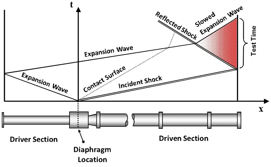
An x-t diagram (shown below) shows this process and depicts the region where the experiment occurs. The horizontal axis indicates position along the shock tube, and the vertical axis shows time elapsed since diaphragm rupture. Near the endwall (the far right in the x-t diagram) of the shock tube is an ideal environment for studying combustion processes at high temperature and pressure. Optical windows and pressure transducers are used in this region to track pressure, emission, and species concentrations in the test gas during the experiment.

Despite their many advantages and applications, several limitations are present when running shock-tube experiments, and a major limitation is the test time. As shown in the x-t diagram above, the test time is defined by the difference between shock wave reflection and the arrival of the expansion wave at the endwall. Several methods can be used to delay the expansion wave arrival, most obvious of which is to extend the driver section. Another method is to slow down the expansion wave by decreasing the sound speed of the driver gas by adding heavier gasses. In our laboratory, the shock tubes are configurable to test times upward of 12 ms.

Other limitations include non-ideal phenomena stemming from viscous effects within the shock tube. These effects depend highly on the test gas and the shock-tube geometry. Due to the relatively large inner diameter of our shock tubes, these viscous effects are minimized compared to other, smaller shock-tube facilities. Investigations have and are continuously being made to characterize and minimize these effects further within these shock tubes, and others, to maximize the data quality. Further information on work done in this laboratory on shock-tube physics is provided in the references below.

Procedure

The procedure involves first importing the .stl file in Converge studio and then flagging boundaries and setting up the case followed by which the case setup is run in cygwin and postprocessed in studio and visualised in paraview.

• First, import the file in studio and then mark the boundaries.
• 
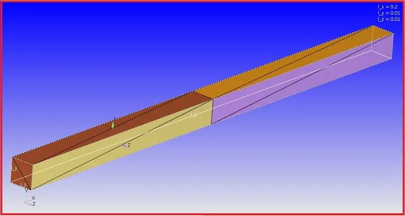
• Next, the face between the two blocks are removed.
• Next, the case is setup and the type of simulation is transient.
• Choose species mode as the type of simulation and setup time parameters.
• 
• 
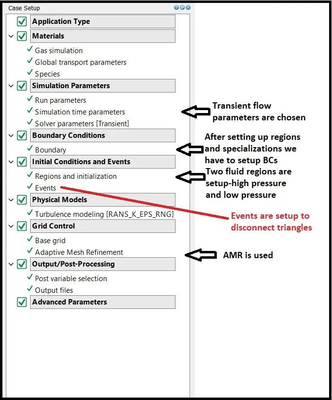
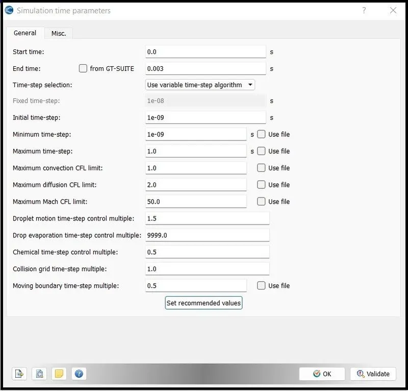
• Once time parameters are setup, the next step is to setup regions and initialize them.
• Two fluid regions are created named 'high pressure' and 'low pressure' region.
• High pressure region is initialised with a pressure of 6 bar while the low pressure region is initialised with a pressure of 1.0132 bar.
• Once done, setup the boundary conditions and set all cases to wall with slip BC and allocate regions to appropriate boundary.
• Once done, setup events.
• 
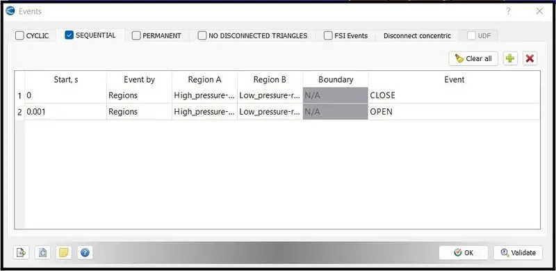
• Here at the start, we set the diaphragm to close(virtual triangle is connected) and at 0.001s, we open the diaphragm(disconnect triangle). Sequential mode is chosen
• Once event is created, create mesh grid size and AMR and select mass fraction and other parameters in the post variable selection window.
• Once done, you should be able to see two regions while turning on group color by region, as shown below.
• 
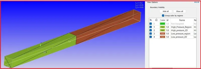
• Export the input files and run the case setup in cygwin.

Results and Discussions

The following are the results and plots and animations showing the variation of parameters like pressure, temperature and celll count as a function of time.

• Let state 1 represent flow properties ahead of compression wave and state 2 represent flow properties behind of compression wave
• Then `underset(02)(P)>underset(01)(P)`
• `underset(02)(T)>underset(01)(T)`
• `underset(2)(V)

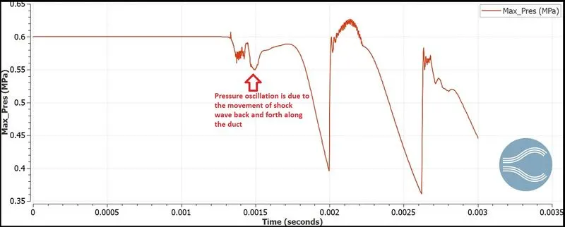
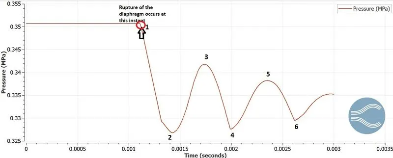
• As shown in the above plots and the video, we see that the pressure drops first and then rises.
• This is due to the fact that in a moving compression wave, the flow region ahead of the compression wave is lower in pressure than behind the wave because the flow behind the wave is compressed.
• Once the shock bounces back, the wavefront will compress already compressed gas thereby rising the pressure.
• Consider the points marked in the figure as the instants where the shock bounces back from the wall.
• Note that 1 is the point at which diaphragm gets ruptured.
• From point 2(which represents the instant at which the shock bounces back, the pressure rises due to the fact that static pressure and total pressure rises across a compression wave by decrement in its absolute velocity.
• The same happens until the wave eventually dies out due to the fact that whenever a wave impinges on a wall and gets reflected, the reflected wave has lower pressure ratio than the impinging wave.
• The mesh generation is also shown here along with the pressure contour.

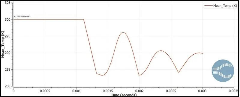
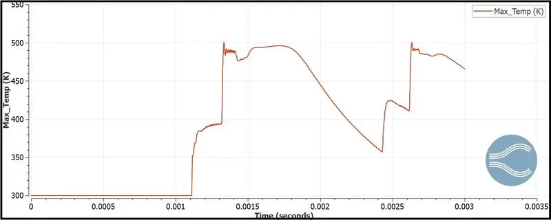
• The same can be explained for temperature variation as well.
• Until the diaphragm gets ruptured, the max temperature remains same.
• Once the diaphragm gets ruptured, the max temperature rises across a compression wave due to the fact that the static and stagnation temperature increases across a compression wave.
• Once shock reflects from the wall, the max temperature drops due to the same reasons as mentioned above.
• Looking at the maximum temperature variation over increasing time, we can see that the due to reflection of shocks, the compression waves rises the temperature even more and then decreases and then increases until the compression wave eventually weakens.
• The mean temperature follows the same trend until the temperature on either side of the shock becomes same.

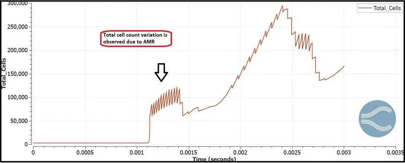
• The above plot shows cell count variation as a function of time.
• Note that until the rupture of the diaphragm, the total number of cells remain constant.
• After the rupture of the diaphragm, the adaptive mesh refinement(AMR) comes into effect.
• The embedding layer is given as 3 which means that the we get three sub divisions of cells.
• The AMR causes the mesh layers to move along with the compression wave thereby indicating presence of compression wave at the location where AMR is found out.

The above shows variation of velocity along a shock tube.

Thus the shock tube simulation is conducted and the results are tabulated.

References

[1] J. W. Hargis and E. L. Petersen, “Shock-Tube Boundary-Layer Effects on Reflected-Shock Conditions With and Without CO₂,” AIAA Journal, Vol. 55, No. 3, 2017, pp. 902-912.

[2] A. R. Amadio, M. W. Crofton, and E. L. Petersen, “Test-Time Extension behind Reflected Shock Waves using CO₂-He and C₃H₈-He Driver Mixtures,” Shock Waves, Vol. 16, No. 2, 2006, pp. 157-165.

[3] E. L. Petersen and R. K. Hanson, “Measurements of Reflected-Shock Bifurcation Over a Wide Range of Gas Composition and Pressure,” Shock Waves, Vol. 15, 2006, pp. 333-340.