Week 3.5 - Deriving 4th order approximation of a 2nd order derivative using Taylor Table method

AIM

To derive the fourth-order approximations of the second-order derivative by following central difference, skewed right side difference, and skewed left side difference schemes and to write a program to determine the error in each case.

DERIVATION

We know that the Taylor's series expansion of a function `f(x)` is

`f(x+a)=f(a)+xf'(a)+x^2/(2!)*f''(a)+...`

For Skewed scheme ,no of nodes=p+q ,where p-> order of derivative q-> order of approximation

Hence,no of nodes=2+4=6 (second-order derivative and 4th order approximation)

For skewed right side scheme: Lets represent second order derivative in a TAYLOR's TABLE

`((d^2u)/dx^2)*Deltax^2 =af(i)+bf(i+1) +cf(i+2)+df(i+3)+ef(i+4)+gf(i+5)`

	f(i)	`Delta xf'(i)`	`Delta x^2f''(i)`	`Delta x^3f'''(i)`	`Delta x^4f''''(i)`	`Delta x^5f'''''(i)`
af(i)	a	0	0	0	0	0
bf(i+1)	b	b	b/2	b/6	b/24	b/120
cf(i+2)	c	2c	4c/2	8c/6	16c/24	32c/120
df(i+3)	d	3d	9d/2	27d/6	81d/24	243d/120
ef(i+4)	e	4e	16e/2	64e/6	256e/24	1024e/120
gf(i+5)	g	5g	25g/2	125g/6	625g/24	3125g/120

Comparing LHS and RHS,

a+b+c+d+e+g=0

0+b+2c+3d+4e+5g=0

b/2+4c/2+9d/2+16e/2+25g/2=1

b/6 +8c/6+27d/6+64e/6+125g/6=0

b/24 +16c/24 +81d/24 +256e/24+ 625g/24=0

b/120 +32c/120 +243d/120 +1024e/120+ 3125g/120=0

Solving these equations in MATLAB, we get a=3.75 b=-12.8333 c=17.83333 d=-13.0000 e=5.0833 g=-.8333

Therefore,the above equation becomes

`((d^2u)/dx^2)*Deltax^2 =3.75f(i)-12.8333f(i+1) +17.8333f(i+2)-13.0f(i+3)+5.0833f(i+4)-.8333f(i+5)`

To solve skewed left side difference scheme,follow the above procedure

`((d^2u)/dx^2)*Deltax^2 =af(i)+bf(i-1) +cf(i-2)+df(i-3)+ef(i-4)+gf(i-5)`

	f(i)	`Delta xf'(i)`	`Delta x^2f''(i)`	`Delta x^3f'''(i)`	`Delta x^4f''''(i)`	`Delta x^5f'''''(i)`
af(i)	a	0	0	0	0	0
bf(i+1)	b	-b	b/2	-b/6	b/24	-b/120
cf(i+2)	c	-2c	4c/2	-8c/6	16c/24	-32c/120
df(i+3)	d	-3d	9d/2	-27d/6	81d/24	-243d/120
ef(i+4)	e	-4e	16e/2	-64e/6	256e/24	-1024e/120
gf(i+5)	g	-5g	25g/2	-125g/6	625g/24	-3125g/120

Solving the above equations,will yield the same values for the constants as above. The eqn becomes

`((d^2u)/dx^2)*Deltax^2 =3.75f(i)-12.8333f(i-1) +17.8333f(i-2)-13f(i-3)+5.0833f(i-4)-0.8333f(i-5)`

To solve central difference scheme for 4th order approximation no of nodes=p+q-1 =2+4-1=5. Hence we require 5 terms

`((d^2u)/dx^2)*Deltax^2 =af(i-2)+bf(i-1) +cf(i)+df(i+1)+ef(i+2)`

	f(i)	`f'(i)`	`f''(i)`	`f'''(i)`	`f''''(i)`
af(i-2)	a	-2a	4a/2	-8a/6	16a/24
bf(i-1)	b	-b	b/2	-b/6	b/24
cf(i)	c	0	0	0	0
df(i+1)	d	d	d/2	d/6	d/24
ef(i+2)	e	2e	4e/2	8e/6	16e/24

In the similar way,upon solving the above equation

a+b+c+d+e=0

-2a-b+d+2e=0

2a+b/2 +d/2 +2e=1

-8a/6 -b/6 +d/6 +8e/6=0

16a/24 +b/24 +d/24 +16e/24=0

we get a=e=-0.0833 b=d=1.3333 c=-2.5

Therefore,the above eqn reduces to

`((d^2u)/dx^2)*Deltax^2 =-0.08333f(i-2)+1.3333f(i-1) -2.5f(i)+1.3333f(i+1)-0.08333f(i+2)`

The above eqns are thus sufficient to write a program to compute the required value

PROGRAM

%This program is for all functions in SOCD,SOSRD,SOSLD
x=pi/3;
dx=linspace(pi/3,pi/3000,160);
for i=1:length(dx)
    error_CD(i)=function_for_SOCD(x,dx(i));
    error_RD(i)=function_for_SOSRD(x,dx(i));
    error_LD(i)=function_for_SOSLD(x,dx(i));
end

%Plotting
figure(1)
loglog(dx,error_CD,'r','linewidth',2);
hold on
loglog(dx,error_RD,'b','linewidth',2);
hold on
loglog(dx,error_LD,'g','linewidth',2);
legend('Central differencing','Skewed Right','Skewed Left');
xlabel('dx');
ylabel('error in each scheme');

The above program is the main program, which is split into small chunks of functions each written for central, skewed left, and right schemes respectively. The value of x is declared, and values of dx are generated over an array. The functions are enclosed inside a loop.

For central difference function:

function[error_CD]=function_for_SOCD(x,dx)
%SOCD->Second order central differencing method for the function
%exp(x)*cos(x)
analyt_deriv=-2*exp(x)*sin(x);    %analytical derivative
%Writing a matrix to solve
a3=[1 1 1 1 1;-2 -1 0 1 2;4/2 1/2 0 1/2 4/2;-8/6 -1/6 0 1/6 8/6;16/24 1/24 0 1/24 16/24];
b3=[0;0;1;0;0];
c3=linsolve(a3,b3);
%Numerical Central differencing scheme
second_deriv_using_central_diff = (((c3(1)*exp(x-(2*dx))*cos(x-(2*dx)))+(c3(2)*exp(x-dx)*cos(x-dx))+(c3(3)*exp(x)*cos(x))+(c3(4)*exp(x+dx))*cos(x+dx))+(c3(5)*exp(x+(2*dx))*cos(x+(2*dx))))/(dx^2);
%error
error_CD=abs(analyt_deriv-second_deriv_using_central_diff);
end

At first, the analytical derivative of the given function is calculated and the matrix is typed and is solved by an inbuilt command linsolve. The formula is inserted for a central difference scheme. The error is calculated as the absolute difference in the analytical expression and the numerical expression. The program is repeated in the same way for skewed cases as well.

For skewed Left-sided difference function:

function[error_LD]=function_for_SOSLD(x,dx)
%SOSLD-> second order skewed left difference scheme for the function exp(x)*cox(x)
%analytical second order derivative of the above function is
analyt_deriv=-2*exp(x)*sin(x);
%Writing the matrix to solve 
a1=[1  1 1 1 1 1 ; 0 -1 -2 -3 -4 -5 ; 0, 1/2,  4/2,  9/2, 16/2, 25/2; 0, -1/6, -8/6, -27/6, -64/6, -125/6; 0, 1/24, 16/24, 81/24, 256/24, 625/24;  0, -1/120, -32/120, -243/120, -1024/120, -3125/120];
b1=[0 ;0;1;0;0;0];
c1=linsolve(a1,b1);
%calculating second order
Derivative_Skewed_left_side = ((c1(1)*exp(x)*cos(x))+(c1(2)*exp(x-dx)*cos(x-dx))+(c1(3)*exp(x-(2*dx))*cos(x-(2*dx)))+(c1(4)*exp(x-(3*dx))*cos(x-(3*dx)))+(c1(5)*exp(x-(4*dx))*cos(x-(4*dx)))+(c1(6)*exp(x-(5*dx))*cos(x-(5*dx))))/(dx^2);
%error
error_LD=abs(analyt_deriv-Derivative_Skewed_left_side);
end

For skewed right-sided difference function:

function[error_RD]=function_for_SOSRD(x,dx)
analyt_deriv=-2*exp(x)*sin(x);
%% Evaluating the coefficients for the right skewed  scheme of 4 order accuracy 
%d^2(f)/dx^2=af(i)+bf(i+1)+cf(i+2)++df(i+3)+ef(i+4)++ff(i+5)
% A total of 6 nodes in the stenscil are required here as per the
% standandard norm specified in the prooblem
a2=[1  1 1 1 1 1 ; 0 1 2 3 4 5 ; 0, 1/2,  4/2,  9/2, 16/2, 25/2; 0, 1/6, 8/6, 27/6, 64/6, 125/6; 0, 1/24, 16/24, 81/24, 256/24, 625/24;  0, 1/120, 32/120, 243/120, 1024/120, 3125/120];
b2=[0 ;0;1;0;0;0];
c2= linsolve(a2,b2);
Derivative_Skewed_right_side = ((c2(1)*exp(x)*cos(x))+(c2(2)*exp(x+dx)*cos(x+dx))+(c2(3)*exp(x+ (2*dx))*cos(x+(2*dx)))+(c2(4)*exp(x+(3*dx))*cos(x+(3*dx)))+(c2(5)*exp(x+(4*dx))*cos(x+(4*dx)))+(c2(6)*exp(x+ (5*dx))*cos(x+(5*dx))))/(dx^2);
error_RD=abs(analyt_deriv-Derivative_Skewed_right_side);

end

Results and Discussions

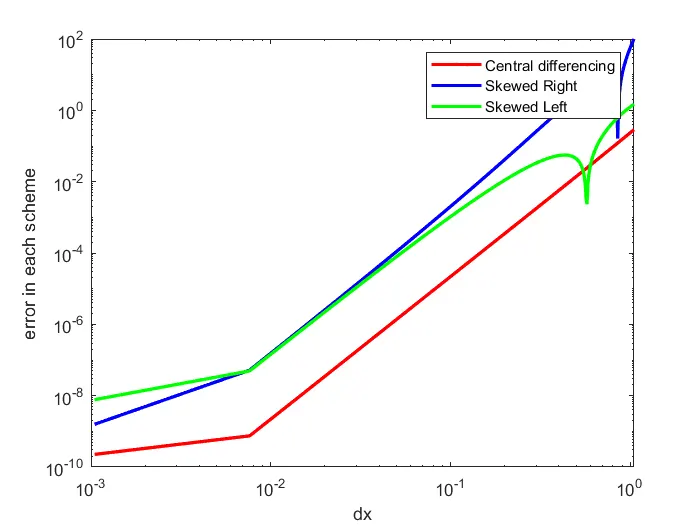
From the above plot, we can infer that the error approaches zero for the central difference scheme whereas the error is closer to zero for the remaining two schemes. Hence a central differencing scheme is useful in these cases. But if the equations were to be solved at the boundary, central difference schemes cant be used. Hence, skewed schemes can be used in such cases.