Project 4
Project 4
In this challenge, we will be running a tutorial from $FOAM_TUTORIALS/compressible/sonicFoam/shockTube and replacing the controlDict, fvSchemes and fvSolutions with that from $FOAM_TUTORIALS/basic/scalarTransportFoam/pitzDaily
Instead of keeping temperatures on one side as high and the other side as low, we will consider a high temperature over a region at the centre of the tube and then solve the governing equations with pure diffusion(Pe->0) and pure advection(Pe->`\infty`).
Copy the shockTube tutorial from the aforementioned directory and replace the controlDict, fvSchemes and fvSolution from that of scalarTransportFoam. Since we are solving for temperature, we need to add an additional transport equation for temperature.
`\frac{\partialT}{\partialt} + (U.\grad)T=\grad.(DT\gradT)`
where DT->diffusion coefficient.
So we will have to make necessary changes to the fvScheme files. We will consider two cases here:
1. We will vary the value of diffusion coefficient(DT) from 0 to 1 keeping the divSchemes constant
2. We will vary the divSchemes keeping the value of diffusion coefficient(DT) constant.
Make copies of the shockTube tutorial for different cases and rename it appropriately. First thing to do is to create a transportProperties file, which can be done by copying one from the pitzDaily case and pasting it in the constant folder.
controlDict file
Here, we will be using scalarTransportFoam controlDict file to run the shocktube case. The solution is run for 5s with a step size of 0.01.
/*--------------------------------*- C++ -*----------------------------------*\
| =========                 |                                                 |
| \\      /  F ield         | OpenFOAM: The Open Source CFD Toolbox           |
|  \\    /   O peration     | Version:  v2206                                 |
|   \\  /    A nd           | Website:  www.openfoam.com                      |
|    \\/     M anipulation  |                                                 |
\*---------------------------------------------------------------------------*/
FoamFile
{
    version     2.0;
    format      ascii;
    class       dictionary;
    object      controlDict;
}
// * * * * * * * * * * * * * * * * * * * * * * * * * * * * * * * * * * * * * //

application     scalarTransportFoam;

startFrom       startTime;

startTime       0;

stopAt          endTime;

endTime         5;

deltaT          0.01;

writeControl    timeStep;

writeInterval   10;

purgeWrite      0;

writeFormat     ascii;

writePrecision  6;

writeCompression off;

timeFormat      general;

timePrecision   6;

runTimeModifiable true;


// ************************************************************************* //
fvSchemes file
In fvSchemes file, we add a gradient scheme and a divergence scheme for temperature by specifying the schemes as shown below. This is the fvScheme file followed for all subcases in case 1.
/*--------------------------------*- C++ -*----------------------------------*\
| =========                 |                                                 |
| \\      /  F ield         | OpenFOAM: The Open Source CFD Toolbox           |
|  \\    /   O peration     | Version:  v2206                                 |
|   \\  /    A nd           | Website:  www.openfoam.com                      |
|    \\/     M anipulation  |                                                 |
\*---------------------------------------------------------------------------*/
FoamFile
{
    version     2.0;
    format      ascii;
    class       dictionary;
    object      fvSchemes;
}
// * * * * * * * * * * * * * * * * * * * * * * * * * * * * * * * * * * * * * //

ddtSchemes
{
    default         Euler;
}

gradSchemes
{
    default         Gauss linear;
    grad(p)         Gauss linear;
    grad(T)         Gauss linear;
}

divSchemes
{
    default         none;

    div(phi,U)      Gauss upwind;

    div(phid,p)     Gauss limitedLinear 1;
    div(phi,e)      Gauss limitedLinear 1;
    div(phi,K)      Gauss limitedLinear 1;
    div(phiv,p)     Gauss limitedLinear 1;
    div(phi,T)      Gauss limitedLinear 1;

    div(((rho*nuEff)*dev2(T(grad(U))))) Gauss linear;
}

laplacianSchemes
{
    default         Gauss linear orthogonal;
}

interpolationSchemes
{
    default         linear;
}

snGradSchemes
{
    default         orthogonal;
}


// ************************************************************************* //
fvSolution file
Because we are solving for temperature, we need to write few lines of code to include a solver for temperature, which is as shown below in the file
/*--------------------------------*- C++ -*----------------------------------*\
| =========                 |                                                 |
| \\      /  F ield         | OpenFOAM: The Open Source CFD Toolbox           |
|  \\    /   O peration     | Version:  v2206                                 |
|   \\  /    A nd           | Website:  www.openfoam.com                      |
|    \\/     M anipulation  |                                                 |
\*---------------------------------------------------------------------------*/
FoamFile
{
    version     2.0;
    format      ascii;
    class       dictionary;
    object      fvSolution;
}
// * * * * * * * * * * * * * * * * * * * * * * * * * * * * * * * * * * * * * //

solvers
{
    "(p|U|e).*"
    {
        solver          smoothSolver;
        smoother        symGaussSeidel;
        tolerance       1e-15;
        relTol          0;
    }

    "rho.*"
    {
        solver          PCG;
        preconditioner  DIC;
        tolerance       1e-15;
        relTol          0;
    }

    T
    {
        solver          PBiCG;
        preconditioner  DILU;
        tolerance       1e-06;
        relTol          0;
    }
}

PIMPLE
{
    nOuterCorrectors     2;
    nCorrectors          1;
    nNonOrthogonalCorrectors 0;
}


// ************************************************************************* //
setFieldsDict file
What the setFieldsDict does is that it declares temperature values over the specified zone as 1 and the remainder of the zones as 0. For case 1, we will consider velocity to be zero.
/*--------------------------------*- C++ -*----------------------------------*\
| =========                 |                                                 |
| \\      /  F ield         | OpenFOAM: The Open Source CFD Toolbox           |
|  \\    /   O peration     | Version:  v2206                                 |
|   \\  /    A nd           | Website:  www.openfoam.com                      |
|    \\/     M anipulation  |                                                 |
\*---------------------------------------------------------------------------*/
FoamFile
{
    version     2.0;
    format      ascii;
    class       dictionary;
    object      setFieldsDict;
}
// * * * * * * * * * * * * * * * * * * * * * * * * * * * * * * * * * * * * * //

defaultFieldValues
(
    volVectorFieldValue U (0 0 0)
    //volScalarFieldValue T 348.432
    volScalarFieldValue T 0.0
    //volScalarFieldValue p 100000
);

regions
(
    boxToCell
    {
        box (-0.5 -1 -1) (0.5 1 1);
        fieldValues
        (
            //volScalarFieldValue T 278.746
            volScalarFieldValue T 1.0
            //volScalarFieldValue p 10000
        );
    }
);
transportProperties file
We copy this file from spitzDaily and vary the value of DT for each case.
/*--------------------------------*- C++ -*----------------------------------*\
| =========                 |                                                 |
| \\      /  F ield         | OpenFOAM: The Open Source CFD Toolbox           |
|  \\    /   O peration     | Version:  v2206                                 |
|   \\  /    A nd           | Website:  www.openfoam.com                      |
|    \\/     M anipulation  |                                                 |
\*---------------------------------------------------------------------------*/
FoamFile
{
    version     2.0;
    format      ascii;
    class       dictionary;
    object      transportProperties;
}
// * * * * * * * * * * * * * * * * * * * * * * * * * * * * * * * * * * * * * //

DT              0.0;


// ************************************************************************* //
Once done, we type in the following commands to run the code:
./Allclean
./Allrun
blockMesh
scalarTransportFoam
foamToVTK(for getting .vtm files so as to view the results in paraview)
Error while executing ./Allrun
If you get an error like ./Allrun: Permission denied, then type in the following commands:
chmod u+x Allrun
chmod u+x Allclean
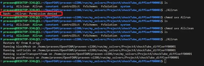
-> If you get floating point exception error, reduce the timestep size.
Results
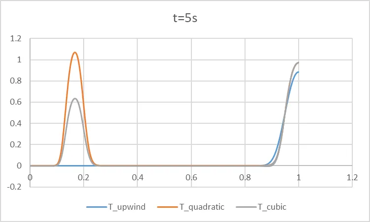
(Plot of Temperature vs length of shock tube for different divSchemes at t=5s)
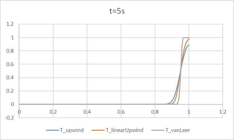
(Plot of Temperature vs length of shock tube for different divSchemes at t=5s)
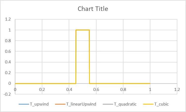
(Plot of Temperature vs length of shock tube for different values of diffusion coefficient at t=0s)
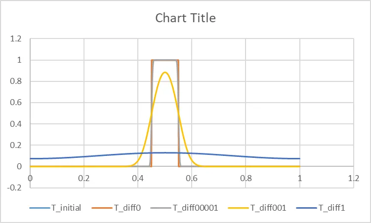
(Plot of Temperature vs length of shock tube for different values of diffusion coefficient at t=5s)
Temperature distribution along the shocktube
| Diffusion Coefficient | Temperature contour |
| 0 | 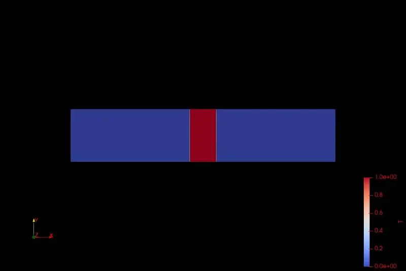 |
| 0.0001 | 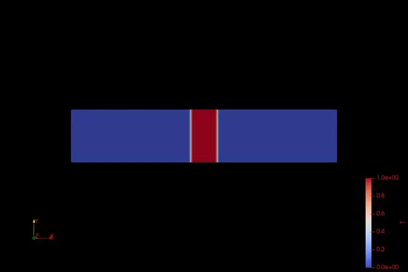 |
| 0.01 | 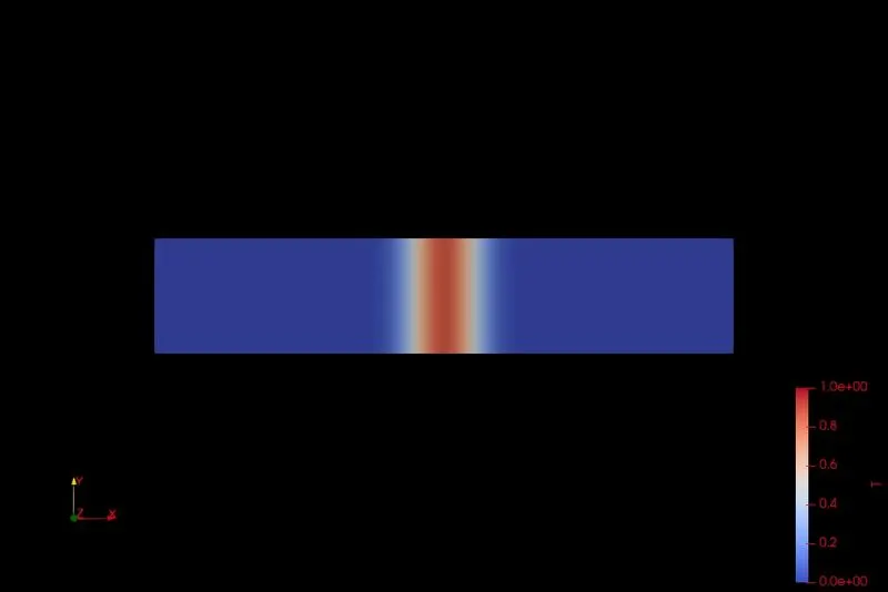 |
| 1 | 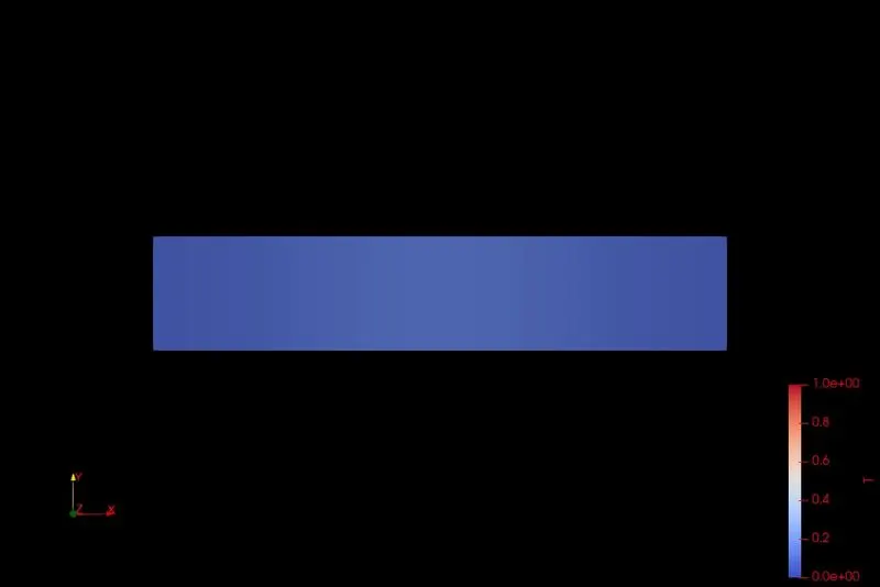 |
| divSchemes | Temperature |
| upwind | 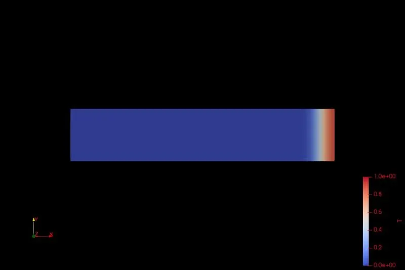 |
| linearUpwind | 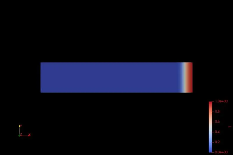 |
| quadraticFit | 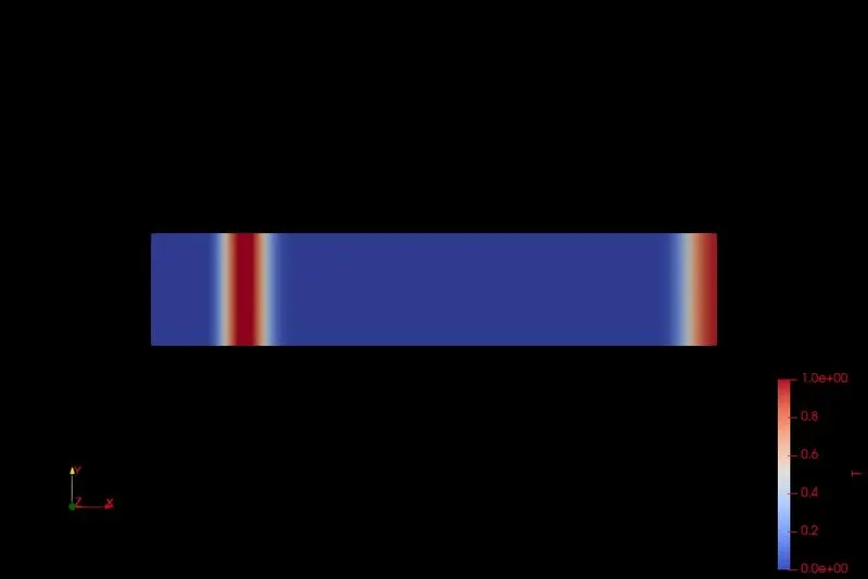 |
| cubic | 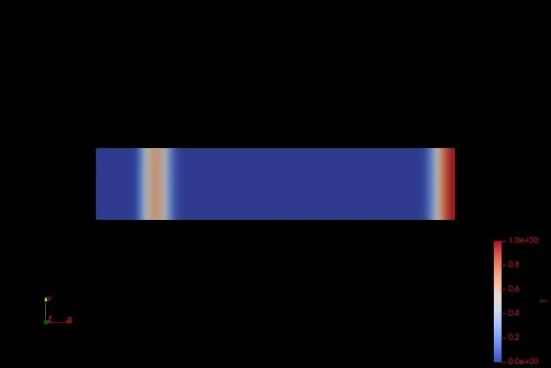 |
| vanLeer | 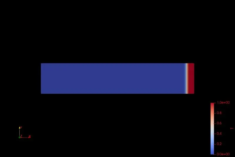 |
Discussions
-> From the above plots, we can see that a diffusion coefficient of 0 results in nothing happening to the temperature i.e, whatever temperature was there before, same is for all times.
-> For a diffusion coefficient of 0.0001, we see that there is a small amount of diffusion(i.e Pe very small), where Peclet number is defined as the ratio of advective effects to diffusive effects. We see that the contours fading slightly at the ends, and if allowed a long period of time, temperature will equilibrate.
-> For a diffusion coefficient of 0.01, the temperature diffuses out much effectively than that for the previous two cases
-> For a diffusion coefficient of 1(which is equivalent to Pe=1 i.e, the convective effects are same as diffusive effects), we see that the temperature has equilibrated throughout the shock tube.
-> The plots above show the diffusive effects for each value of diffusion coefficient
-> We also have compared plots for different divergent schemes, as shown above.
-> We can see that the vanLeer scheme is the most accurate scheme compared to the other schemes,because it closely resembles the ideal case.
-> The basic upwinding scheme is the most stable and unconditionally bound scheme, but it introduces a high level of false diffusion due to its lower order of accuracy(first-order).
-> Higher order schemes, such as central differencing and QUICK can give spurious oscillations when the Peclet number is high.
-> When such higher order schemes are used to solve for turbulent quantities like dissipation, wiggles can give physically unrealistic negative values and instability.
->vanLeer is a TVD(total variation diminishing) scheme designed to address this oscillation. In TVDm tendency towards oscillation is counteracted by adding an artificial diffusion fragment or by adding a weighting towards upstream contribution.
-> The accuracy of upwind schemes is only first order in terms of taylor series truncation error. The use of upwind quantities ensures that the schemes are very stable and obey the transportiveness requirement, but the first order accuracy makes them prone to numerical diffusion errors.
-> Such errors can be minimised by employing higher order discretisation, which involve more neighbouring points and reduce the discretisation errors by bringing in a wider influence.
LATEX code
\documentclass[12pt]{report}
\usepackage{graphicx} % Required for inserting images
\usepackage{amsfonts,amsmath,amssymb}
\usepackage[margin=1in]{geometry}
\usepackage[inline]{enumitem}
\usepackage{float}
\usepackage{fancyhdr}

\pagestyle{fancy}
\fancyhead{}
\fancyfoot{}
\fancyhead[L]{Project4}
\fancyhead[R]{OpenFOAM}
\fancyfoot[C]{\thepage}
\renewcommand{\footrulewidth}{0.4pt}% Default \footrulewidth is 0pt
\renewcommand{\headrulewidth}{0.4pt}% Default \headrulewidth is 0.4pt


\begin{document}
\begin{center}
    \section*{Comparison of discretisation schemes and diffusion coefficients for a case of shock tube in OpenFOAM}
    \section*{Abstract}
\end{center}
In this challenge, we will be running a tutorial from \\ $\mathtt{FOAMTUTORIALS/compressible/sonicFoam/shockTube}$ and replacing the controlDict, fvSchemes and fvSolutions with that from \\ $\mathtt{FOAMTUTORIALS/basic/scalarTransportFoam/pitzDaily}$\\

Instead of keeping temperatures on one side as high and the other side as low, we will consider a high temperature over a region at the centre of the tube and then solve the governing equations with pure diffusion(Pe-0) and pure advection(Pe-$\infty$).

Copy the shockTube tutorial from the aforementioned directory and replace the controlDict, fvSchemes and fvSolution from that of scalarTransportFoam. Since we are solving for temperature, we need to add an additional transport equation for temperature.

$$\frac{\partial T}{\partial t} + (U.\nabla) T= \nabla.(DT\nabla T)$$

where DT-diffusion coefficient.

So we will have to make necessary changes to the fvScheme files.

\section*{Procedure}
We will consider two cases here:
\begin{enumerate}
    \item We will vary the value of diffusion coefficient(DT) from 0 to 1 keeping the divSchemes constant.
    \item We will vary the divSchemes keeping the value of diffusion coefficient(DT) constant.
\end{enumerate}

Make copies of the shockTube tutorial for different cases and rename it appropriately. First thing to do is to create a \texttt{transportProperties} file, which can be done by copying one from the pitzDaily case and pasting it in the constant folder.

\section*{Changes to the files}
\subsection*{controlDict}
Here, we will be using scalarTransportFoam controlDict file to run the shocktube case. The solution is run for 5s with a step size of 0.01.

\begin{verbatim}
    /*--------------------------------*- C++ -*----------------------------------*\
| =========                 |                                                 |
| \\      /  F ield         | OpenFOAM: The Open Source CFD Toolbox           |
|  \\    /   O peration     | Version:  v2206                                 |
|   \\  /    A nd           | Website:  www.openfoam.com                      |
|    \\/     M anipulation  |                                                 |
\*---------------------------------------------------------------------------*/
FoamFile
{
    version     2.0;
    format      ascii;
    class       dictionary;
    object      controlDict;
}
// * * * * * * * * * * * * * * * * * * * * * * * * * * * * * * * * * * * * * //

application     scalarTransportFoam;

startFrom       startTime;

startTime       0;

stopAt          endTime;

endTime         5;

deltaT          0.01;

writeControl    timeStep;

writeInterval   10;

purgeWrite      0;

writeFormat     ascii;

writePrecision  6;

writeCompression off;

timeFormat      general;

timePrecision   6;

runTimeModifiable true;


// ************************************************************************* //
\end{verbatim}

\subsection*{fvSchemes}
In fvSchemes file, we add a gradient scheme and a divergence scheme for temperature by specifying the schemes as shown below. This is the fvScheme file followed for all subcases in case 1.

\begin{verbatim}
    /*--------------------------------*- C++ -*----------------------------------*\
| =========                 |                                                 |
| \\      /  F ield         | OpenFOAM: The Open Source CFD Toolbox           |
|  \\    /   O peration     | Version:  v2206                                 |
|   \\  /    A nd           | Website:  www.openfoam.com                      |
|    \\/     M anipulation  |                                                 |
\*---------------------------------------------------------------------------*/
FoamFile
{
    version     2.0;
    format      ascii;
    class       dictionary;
    object      fvSchemes;
}
// * * * * * * * * * * * * * * * * * * * * * * * * * * * * * * * * * * * * * //

ddtSchemes
{
    default         Euler;
}

gradSchemes
{
    default         Gauss linear;
    grad(p)         Gauss linear;
    grad(T)         Gauss linear;
}

divSchemes
{
    default         none;

    div(phi,U)      Gauss upwind;

    div(phid,p)     Gauss limitedLinear 1;
    div(phi,e)      Gauss limitedLinear 1;
    div(phi,K)      Gauss limitedLinear 1;
    div(phiv,p)     Gauss limitedLinear 1;
    div(phi,T)      Gauss limitedLinear 1;

    div(((rho*nuEff)*dev2(T(grad(U))))) Gauss linear;
}

laplacianSchemes
{
    default         Gauss linear orthogonal;
}

interpolationSchemes
{
    default         linear;
}

snGradSchemes
{
    default         orthogonal;
}


// ************************************************************************* //

\end{verbatim}

\subsection*{fvSolution}
Because we are solving for temperature, we need to write few lines of code to include a solver for temperature, which is as shown below in the file

\begin{verbatim}
    /*--------------------------------*- C++ -*----------------------------------*\
| =========                 |                                                 |
| \\      /  F ield         | OpenFOAM: The Open Source CFD Toolbox           |
|  \\    /   O peration     | Version:  v2206                                 |
|   \\  /    A nd           | Website:  www.openfoam.com                      |
|    \\/     M anipulation  |                                                 |
\*---------------------------------------------------------------------------*/
FoamFile
{
    version     2.0;
    format      ascii;
    class       dictionary;
    object      fvSolution;
}
// * * * * * * * * * * * * * * * * * * * * * * * * * * * * * * * * * * * * * //

solvers
{
    "(p|U|e).*"
    {
        solver          smoothSolver;
        smoother        symGaussSeidel;
        tolerance       1e-15;
        relTol          0;
    }

    "rho.*"
    {
        solver          PCG;
        preconditioner  DIC;
        tolerance       1e-15;
        relTol          0;
    }

    T
    {
        solver          PBiCG;
        preconditioner  DILU;
        tolerance       1e-06;
        relTol          0;
    }
}

PIMPLE
{
    nOuterCorrectors     2;
    nCorrectors          1;
    nNonOrthogonalCorrectors 0;
}


// ************************************************************************* //

\end{verbatim}

\subsection*{setFields}
What the setFieldsDict does is that it declares temperature values over the specified zone as 1 and the remainder of the zones as 0. For case 1, we will consider velocity to be zero.

\begin{verbatim}
    /*--------------------------------*- C++ -*----------------------------------*\
| =========                 |                                                 |
| \\      /  F ield         | OpenFOAM: The Open Source CFD Toolbox           |
|  \\    /   O peration     | Version:  v2206                                 |
|   \\  /    A nd           | Website:  www.openfoam.com                      |
|    \\/     M anipulation  |                                                 |
\*---------------------------------------------------------------------------*/
FoamFile
{
    version     2.0;
    format      ascii;
    class       dictionary;
    object      setFieldsDict;
}
// * * * * * * * * * * * * * * * * * * * * * * * * * * * * * * * * * * * * * //

defaultFieldValues
(
    volVectorFieldValue U (0 0 0)
    //volScalarFieldValue T 348.432
    volScalarFieldValue T 0.0
    //volScalarFieldValue p 100000
);

regions
(
    boxToCell
    {
        box (-0.5 -1 -1) (0.5 1 1);
        fieldValues
        (
            //volScalarFieldValue T 278.746
            volScalarFieldValue T 1.0
            //volScalarFieldValue p 10000
        );
    }
);
\end{verbatim}

\subsection*{transportProperties}
We copy this file from spitzDaily and vary the value of DT for each case.


\begin{verbatim}
    /*--------------------------------*- C++ -*----------------------------------*\
| =========                 |                                                 |
| \\      /  F ield         | OpenFOAM: The Open Source CFD Toolbox           |
|  \\    /   O peration     | Version:  v2206                                 |
|   \\  /    A nd           | Website:  www.openfoam.com                      |
|    \\/     M anipulation  |                                                 |
\*---------------------------------------------------------------------------*/
FoamFile
{
    version     2.0;
    format      ascii;
    class       dictionary;
    object      transportProperties;
}
// * * * * * * * * * * * * * * * * * * * * * * * * * * * * * * * * * * * * * //

DT              0.0;


// ************************************************************************* //
\end{verbatim}

Once done, we type in the following commands to run the code:

\texttt{./Allclean}

\texttt{./Allrun}

\texttt{blockMesh}

\texttt{scalarTransportFoam}

\texttt{foamToVTK}(for getting .vtm files so as to view the results in paraview)

\subsection*{Errors}
\begin{figure}[H]
    \centering
    \includegraphics[width=18cm]{bash_error.jpg}
    \caption{Errors}
    \label{fig:my_label}
\end{figure}

If you get an error like ./Allrun: Permission denied, then type in the following commands:

\texttt{chmod u+x Allrun}

\texttt{chmod u+x Allclean}

If you get floating point exception error, reduce the timestep size.

\section*{Results}
\begin{figure}[H]
    \centering
    \includegraphics[width=12cm]{0.jpg}
    \caption{Plot of Temperature vs length of shock tube for different values of diffusion coefficient at t=0s}
    \label{fig:my_label}
\end{figure}

\begin{figure}[H]
    \centering
    \includegraphics[width=12cm]{3.jpg}
    \caption{Plot of Temperature vs length of shock tube for different values of diffusion coefficient at t=5s}
    \label{fig:my_label}
\end{figure}

\begin{figure}[H]
    \centering
    \includegraphics[width=12cm]{1.jpg}
    \caption{Plot of Temperature vs length of shock tube for different divSchemes at t=5s}
    \label{fig:my_label}
\end{figure}

\begin{figure}[H]
    \centering
    \includegraphics[width=12cm]{2.jpg}
    \caption{Plot of Temperature vs length of shock tube for different divSchemes at t=5s}
    \label{fig:my_label}
\end{figure}
\pagebreak

\subsection*{Temperature distribution along the shocktube}

\begin{figure}[H]
    \centering
    \includegraphics[width=12cm]{T0.jpeg}
    \caption{Diffusion coefficient:0}
    \label{fig:my_label}
\end{figure}

\begin{figure}[H]
    \centering
    \includegraphics[width=12cm]{T00001.jpeg}
    \caption{Diffusion coefficient:0.0001}
    \label{fig:my_label}
\end{figure}

\begin{figure}[H]
    \centering
    \includegraphics[width=12cm]{T001.jpeg}
    \caption{Diffusion coefficient:0.01}
    \label{fig:my_label}
\end{figure}

\begin{figure}[H]
    \centering
    \includegraphics[width=12cm]{T1.jpeg}
    \caption{Diffusion coefficient:1}
    \label{fig:my_label}
\end{figure}

\begin{figure}[H]
    \centering
    \includegraphics[width=12cm]{T_up.jpeg}
    \caption{divScheme: Gauss upwind}
    \label{fig:my_label}
\end{figure}

\begin{figure}[H]
    \centering
    \includegraphics[width=12cm]{TlU.jpeg}
    \caption{divScheme: Gauss linearUpwind}
    \label{fig:my_label}
\end{figure}

\begin{figure}[H]
    \centering
    \includegraphics[width=12cm]{T_quad.jpeg}
    \caption{divScheme: Gauss quadraticFit}
    \label{fig:my_label}
\end{figure}

\begin{figure}[H]
    \centering
    \includegraphics[width=12cm]{T_cub.jpeg}
    \caption{divScheme: Gauss cubic}
    \label{fig:my_label}
\end{figure}

\begin{figure}[H]
    \centering
    \includegraphics[width=12cm]{t_vanLeer.jpeg}
    \caption{divScheme: Gauss vanLeer}
    \label{fig:my_label}
\end{figure}

\section*{Discussions}
\begin{itemize}
    \item From the above plots, we can see that a diffusion coefficient of 0 results in nothing happening to the temperature i.e, whatever temperature was there before, same is for all times.
    \item For a diffusion coefficient of 0.0001, we see that there is a small amount of diffusion(i.e Pe very small), where Peclet number is defined as the ratio of advective effects to diffusive effects. We see that the contours fading slightly at the ends, and if allowed a long period of time, temperature will equilibrate.
    \item For a diffusion coefficient of 0.01, the temperature diffuses out much effectively than that for the previous two cases.
    \item For a diffusion coefficient of 1(which is equivalent to Pe=1 i.e, the convective effects are same as diffusive effects), we see that the temperature has equilibrated throughout the shock tube.
    \item The plots above show the diffusive effects for each value of diffusion coefficient
    \item We also have compared plots for different divergent schemes, as shown above.
    \item We can see that the vanLeer scheme is the most accurate scheme compared to the other schemes,because it closely resembles the ideal case.
    \item The basic upwinding scheme is the most stable and unconditionally bound scheme, but it introduces a high level of false diffusion due to its lower order of accuracy(first-order).
    \item Higher order schemes, such as central differencing and QUICK can give spurious oscillations when the Peclet number is high.
    \item When such higher order schemes are used to solve for turbulent quantities like dissipation, wiggles can give physically unrealistic negative values and instability.
    \item vanLeer is a TVD(total variation diminishing) scheme designed to address this oscillation. In TVDm tendency towards oscillation is counteracted by adding an artificial diffusion fragment or by adding a weighting towards upstream contribution.
    \item The accuracy of upwind schemes is only first order in terms of taylor series truncation error. The use of upwind quantities ensures that the schemes are very stable and obey the transportiveness requirement, but the first order accuracy makes them prone to numerical diffusion errors.
    \item Such errors can be minimised by employing higher order discretisation, which involve more neighbouring points and reduce the discretisation errors by bringing in a wider influence.
\end{itemize}
Thus the discretization schemes are compared and comparison studies are carried out.
\end{document}