Week 3 - External flow simulation over an Ahmed body.
Challenge
In this challenge, an ahmed body is simulated in FLUENT at a velocity of 25m/s with the default air properties. As the body is perfectly symmetric, we can run the simulation by considering the only half body. This is the best practice where we can save on the number of cells and get the results faster as well. The importance of Ahmed body is explained, followed by detailed procedure that was performed in fluent.
The following details are of interest:
1. Contours of Velocity and pressure .
2. The drag coefficient plot for a refined case.
3. The vector plot clearly showing the wake region.
4. Perform the grid independency test and provide the values of drag and lift with each case.
Ahmed Body:
As the burning of fossil fuels becomes a more pressing issue, manufacturers are introducing more fuel efficient cars to the market. One main contributor to fuel burn is the car’s aerodynamic drag. Complexly shaped, cars are very challenging to model and it’s difficult to quantify the aerodynamic drag computationally. The Ahmed body is a benchmark model widely used in the automotive industry for validating simulation tools. The Ahmed body shape is simple enough to model, while maintaining car-like geometry features.
The Ahmed body is a generic car body (a simplified vehicle model). The airflow around the Ahmed body captures the essential flow features around an automobile and was first defined and characterized in the experimental work of Ahmed. Although it has a very simple shape, Ahmed body allows us to capture characteristic features that are relevant to bodies in the automobile industry.
This model is also used to describe the turbulent flow field around a car-like geometry. Once the numerical model in validated, it is used to design new models of the car. Since then, it has become a benchmark for aerodynamic simulation tools. +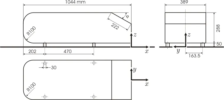
Why study the Drag coefficient in automobiles?
The drag coefficient quantifies the resistance of an object in a fluid environment. It is not an absolute constant for a body’s shape because it varies with the speed and direction of flow, object shape and size, and the density and viscosity of the fluid. The lower the drag coefficient of an object, the less aerodynamic or hydrodynamic drag occurs. In terms of a car, the lower the drag coefficient, the more efficient the car is. As well as affecting the top speed of a vehicle, the drag coefficient also affects the handling. Cars with a low drag coefficient are sought after, but decreasing the drag drastically can reduce the downforce and lead to loss in road traction and a higher chance of car accidents.
Most cars have an average drag coefficient between .30 and .35. The exact drag coefficient of a car varies with the Reynolds number and various other factors.
There are certain ways to modify a car to optimize its aerodynamics and decrease the drag coefficient. To streamline the exterior, you can remove certain aftermarket items such as the roof rack, mud flaps, spoilers, and radio antenna. Professional car racers also take off their windshield wipers and side mirrors, but this isn’t recommended for the average driver! You can also add wheel covers, a partial grille block, an under tray, fender skirts, and a modified front bumper to improve the drag coefficient and make your car stand out in the process.
Setting up the case in Ansys
To setup the flow over an ahmed body, we divide the process into preprocessing, solving and post processing.
In preprocessing, the geometry is fiddled with and necessary alterations are made so as to match the needs and to get accurate solutions. This is followed by meshing in which we divide the entire flow domain into finite volumes so that the equations are solved at the centroid of each volume.
In solving(processing) we give boundary conditions to the solver and turn on the viscous model to k-omega and then run for a set of iterations and create output parameters so as to run grid dependence test.
Geometry
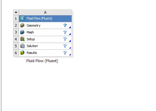
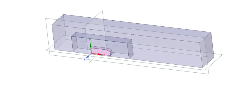
Open the workbench and drag and drop fluent module into the project schematic window. Double click on Geometry and a new spaceclaim window is opened. We need to solve equation around the body, so first import the body and go to prepare menu and click on enclosure. Enter the specified dimensions and hit ok. To make sure that the mesh around the ahmed body is much finer than the enclosure, we have to perform local refinement by drawing another box(enclosure) with smaller dimensions closer to the body. Suppress the body for meshing.

Right click on meshing.This will open up a new window.
To check the base mesh generated by ansys, hit generate button. This will generate a non-uniform mesh.
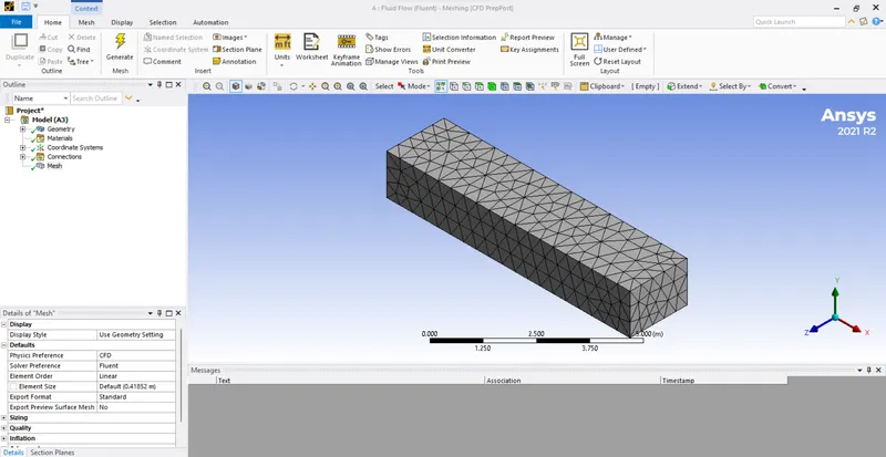
Note that the mesh is irregular and uneven. To make sure that the mesh is fine, right click on mesh and insert method. Select multizone, this will generate hex mesh which is the most efficient mesh amongst all of them.
After meshing, the mesh looks like this
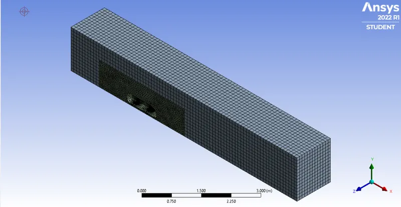
which looks a lot finer than the previous mesh. Name the boundaries. Applying the inflation layers,it should look something as below.
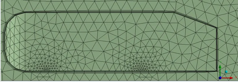
In the left pane, click the checkbox that is available under the defaults menu, so as to perform grid independence test. This will serve as out input parameter for changing values.
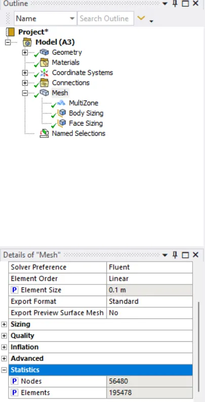
Update the mesh and close it.
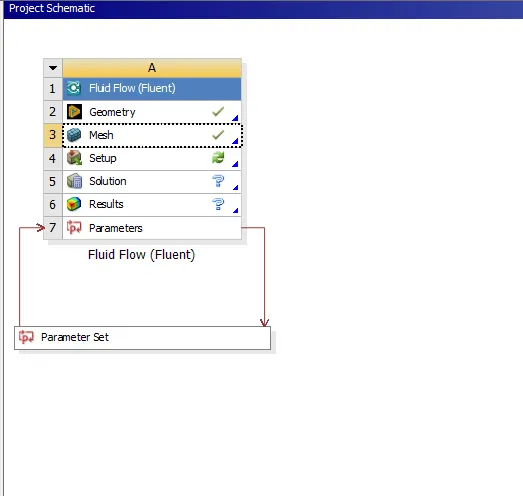
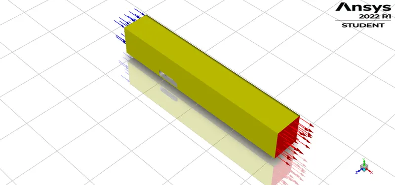
The next step is solving. This involves giving boundary conditions and solving the equations. At first, click on double precision and this will launch fluent.
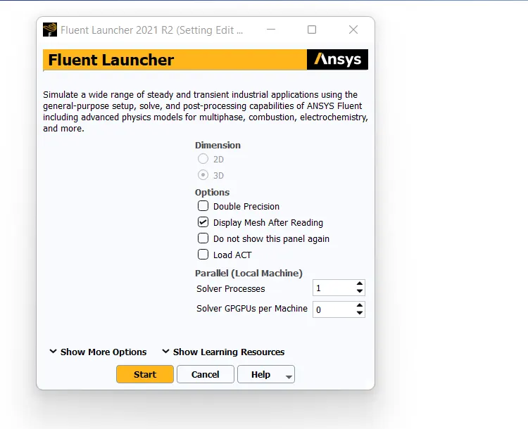
Inside the fluent ,we specify the type of solver to be density based solver. 
Using several options listed above, we have to specify the physics of the domain. Specify the viscous model as K-omega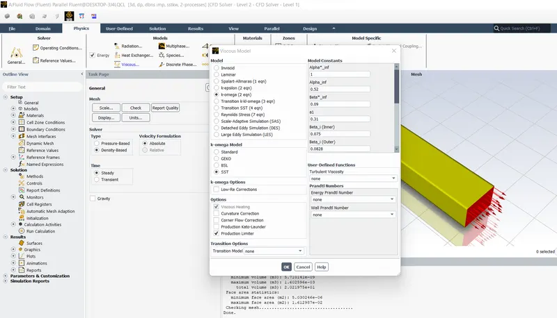
Next, specify the material properties as that of air
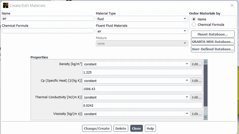
Specify the boundary conditions as well
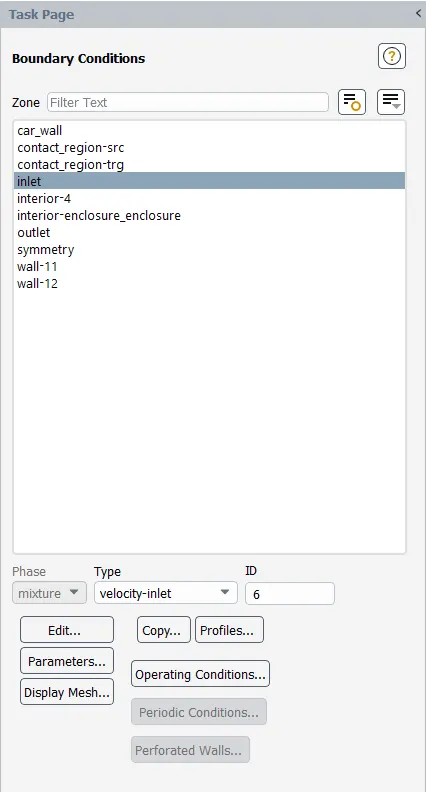
Once it is done, initialize the solution and solve for a set of iterations. The results will converge after some number of iterations.
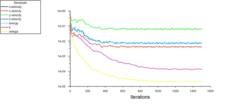
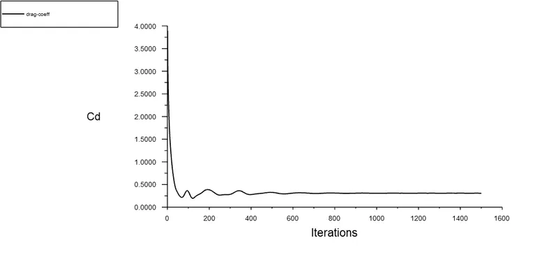
Convergence of drag coefficient value
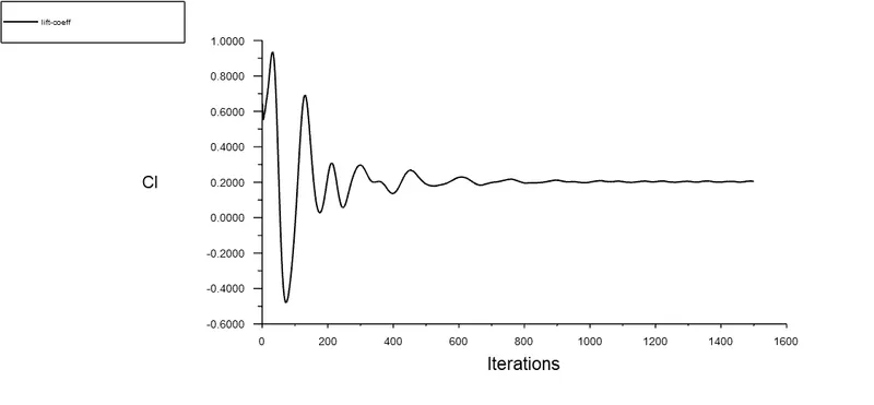
Convergence of lift coefficient value
The next step is to perform post processing analysis of the results that are obtained. Right click on CFD post and click ok.
In this stage, we try to understand the results by drawing plots and getting the values of drag and lift coefficients respectively.
Click on location->plane and create a new plane at the centre of the body on which the velocity contours need to be created. Next click on vectors and plot it for velocity. With this the post processing setup is done.
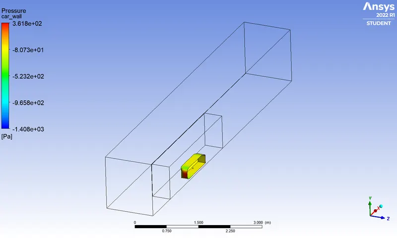
Pressure variation over the entire ahmed body
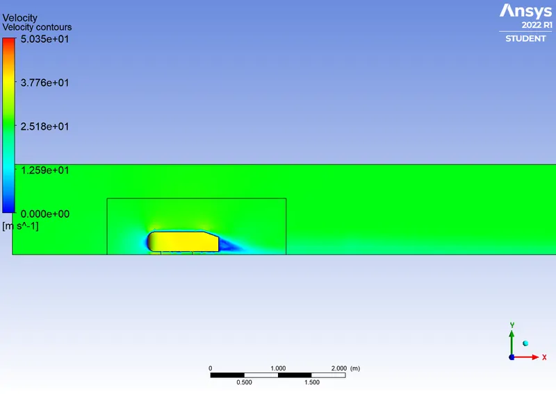
Velocity contour over the ahmed body on a cut plane(without inflation)
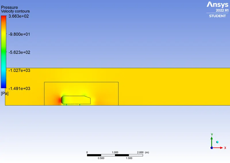
Pressure contour over the ahmed body on a cut plane(without inflation)
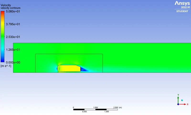
Velocity contour over the ahmed body on a cut plane(with inflation)
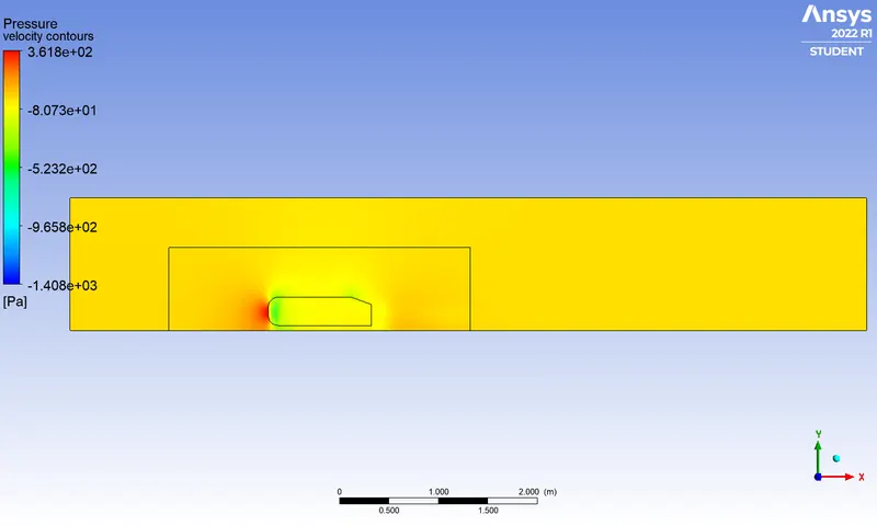
Pressure contour over the ahmed body on a cut plane(with inflation)
The stark contrast between a inflated region and non inflated region is that the former provides better contour as compared to the latter.
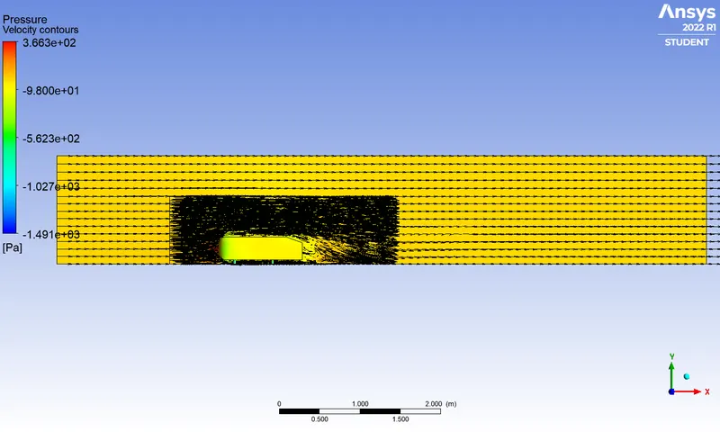
Vector plots of velocity over the ahmed body
The pressure on the front face is maximum, which implies that the pressure measured is the stagnation pressure. Stagnation pressure is defined as the pressure at which the velocity of the fluid is zero.i.e the fluid is slowed down to zero velocity. The wake behind the body indicates that the flow velocity is zero.
Significance of point of separation:
In the external flow over a body, a boundary layer is developed very adjacent to the solid boundary across which viscous effects are predominant. In a flow, there exists two types of pressure gradients-favourable pressure gradient and adverse pressure gradient. The entire ahmed body can be treated as a combination of a viscous flow closer to the body and inviscid flow away from the body.
Favorable pressure gradient is one in which `(delp)/(delx)<0` i.e the flow gets accelerated along the length.
Adverse pressure gradient is one in which `(delp)/(delx)>0` i.e the flow gets decelerated along the length.
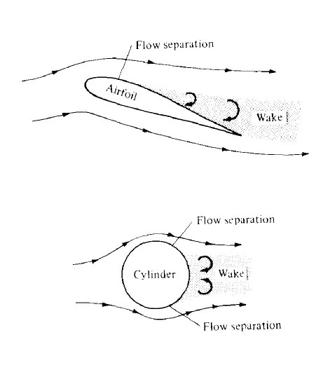
At the point of separation, the shear stresss becomes zero which means the flow gets detached from the surface, leaving behind a recirculation zone called as a wake. The larger the wake, the larger the pressure drag. Aerodynamic designs involve placing this point of separation as far as possible from the leading end of the body. At the point of separation, the flow converts from favorable pressure gradient to adverse pressure gradient. If the favourable pressure gradient is not maintained, the adverse gradient develops which will cause the flow to be chaotic and hence it is highly unfavorable.
Negative Pressure in the wake region
We know that absolute pressure=atmospheric pressure + gauge pressure.
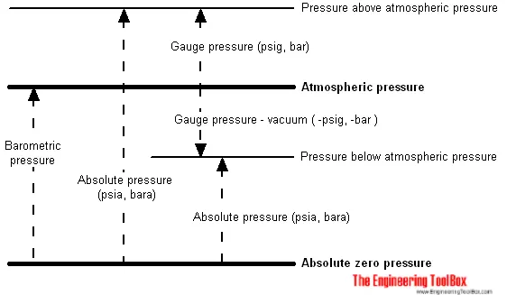
When ansys measures the value of pressure, it measures gauge pressure rather than absolute pressure(which is the sum) and hence we see that the values are negative, which implies that the measured pressure has fallen below atmospheric pressure, which is evident from the figure above. Why does the gauge pressure fall below the atmospheric pressure? As the flow leaves the body(since it is a bluff body) , it leaves at a point called point of separation as discussed above. If the point of separation is delayed by suitable techniques, the flow remains attached to the surface. But because the flow has separated from the surface, the pressure drops below the atmospheric value and hence we get the value as negative one.
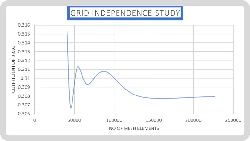
GRID INDEPENDENCY TEST FOR DRAG
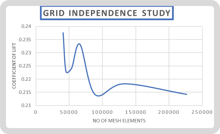
GRID INDEPENDENCY TEST FOR LIFT
VALUES OF CD AND CL
| Mesh nodes | Mesh elements | Coefficient of Drag | Coefficient of Lift |
| 40828 | 118327 | 0.315374 | 0.23766 |
| 45192 | 122056 | 0.306721 | 0.222957 |
| 53690 | 129683 | 0.311251 | 0.224249 |
| 66208 | 141151 | 0.309319 | 0.23323 |
| 88705 | 162168 | 0.310775 | 0.214213 |
| 132722 | 203379 | 0.307949 | 0.218276 |
| 226282 | 291932 | 0.30795 | 0.214269 |
(The values in bold correspond to the refined case.)