Week 8 - Simulating Cyclone separator with Discrete Phase Modelling
Simulating Cyclone separator with Discrete Phase Modelling
| Table Of Contents |
| 1. Aim |
| 2. Theory |
| 3. Procedure |
| 4. Results |
| 5. Animation videos |
| 6. Conclusions |
Aim:
1. To perform analysis on cyclone separator and calculate the separation efficiency and pressure drop.
2. To write a few words about any four empirical models used to calculate the cyclone separator efficiency.
3. To perform an analysis on a given cyclone separator model by varying the particle diameter from 1 μm to 5 μm and
calculate the separation efficiency in each case and also discuss the results for each case.
4. To perform an analysis on a given cyclone separator model by varying the particle velocity from 1 m/sec to 5 m/sec and
calculate the separation efficiency and pressure drop in each case and discuss the results.
Theory:
A cyclone separator is an economical device for removing particulate solids from a fluid system. The induced centrifugal force is tangentially imparted on the wall of the cyclone cylinder. This force, with the density difference between the fluid and solid, increases the relative settling velocity.
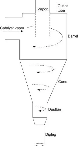
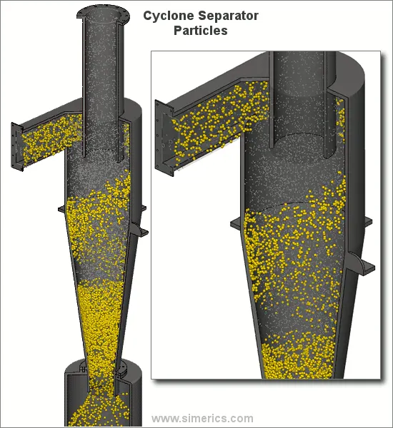
It uses the principle of inertia to remove particulate matter from flue gases.Cyclone separators is one of many air pollution control devices known as precleaners since they generally remove larger pieces of particulate matter. This prevents finer filtration methods from having to deal with large, more abrasive particles later on. In addition, several cyclone separators can operate in parallel, and this system is known as a multicyclone.
It is important to note that cyclones can vary drastically in their size. The size of the cyclone depends largely on how much flue gas must be filtered, thus larger operations tend to need larger cyclones. For example, several different models of one cyclone type can exist, and the sizes can range from a relatively small 1.2-1.5 meters tall (about 4-5 feet) to around 9 meters (30 feet)—which is about as tall as a three story building.
Cyclone separators are generally able to remove somewhere between 50-99% of all particulate matter in flue gas. How well the cyclone separators are actually able to remove this matter depends largely on particle size. If there is a large amount of lighter particulate matter, less of these particles are able to be separated out. Because of this, cyclone separators work best on flue gases that contain large amounts of big particulate matter.
Cyclone separators are extremely important toward the successful operation of the cat cracker. Their performance impacts several FCC performance factors, including the additional cost of fresh catalyst makeup, extra turnaround maintenance costs, the allowable limits on emission of particulates, and the incremental energy recovery in the WGC, and hot gas expander.
Designing an “optimum” set of cyclones requires a balance between the desired collection efficiency, pressure drop, space limitations, and installation cost.
There are several advantages and disadvantages in using cyclone separators. First, cyclone separators are beneficial because they are not expensive to install or maintain, and they have no moving parts. This keeps maintenance and operating costs low. Second, the removed particulate matter is collected when dry, which makes it easier to dispose of. Finally, these units take up very little space. Although effective, there are also disadvantages in using cyclone separators. Mainly because the standard models are not able to collect particulate matter that is smaller than 10 micrometers effectively and the machines are unable to handle sticky or tacky materials well.
Cyclone separation efficiency is defined as the ratio of total number of particles trapped to the total number of particles tracked.
Models to calculate cyclone separator efficiency:
Cyclone separation efficiency is defined as the ratio of total number of particles trapped to the total number of particles tracked.
To define the cyclone separator efficiency, several models have been predicted and are found to agree with the experimental results.
1. Koch and Licht Model
Koch and Licht collection theory recognized the inherently turbulent nature of cyclones and the distribution of gas residence times within the cyclone. Koch and Licht described particle motion in the entry and collection regions with the additional following assumption:
->The tangential velocity of a particle is equal to the tangential velocity of the gas flow, i.e. there is no slip in the tangential direction between the particle and the gas.
-> The tangential velocity is related to the radius of the cyclone as `u*R^n`=constant
2. Li and Wang Model
The Li and Wang model includes particle bounce or re-entrainment and turbulent diffusion at the cyclone wall. A two-dimensional analytical expression of particle distribution in the cyclone is obtained. Li and Wang model was developed based on the following assumption:
->The radial particle velocity and the radial concentration profile are not constant for uncollected particles within the cyclone.
-> The tangential velocity is related to the radius of the cyclone as `u*R^n`=constant
3. Iozia and Leith Model
The Iozia and Leith [4] logistic model is a modified version of Barth [15] Model, which is developed based on force balance.
The model assumes that a particle carried by the vortex endures 165 the influence of two forces: a centrifugal force, Z and a flow resistance, W. The collection efficiency `eta` of particle diameter dpi can be calculated from
`eta=1/(1+(underset(pc)(d)/underset(pi)(d))^beta)`
where `beta`is an empirical data.
4. Lapple Model
The Lapple model was developed based on force balance without considering the flow resistance. Lapple assumed that a particle entering the cyclone is evenly distributed across the inlet opening. The particle that travels from inlet half width to the
wall in the cyclone is collected with 50% efficiency.
Procedure:
The procedure involves first importing the geometry into spaceclaim, then extracting the fluid volume from the model and suppressing the model for physics. The next step involves meshing the geometry and then setting up fluent solver with the necessary conditions so as to simulate particle tracking and creating animation files as well.
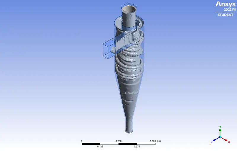
First, the CAD file is imported in spaceclaim. Then the fluid volume is extracted by going to prepare->volume extract. The final product looks like this.
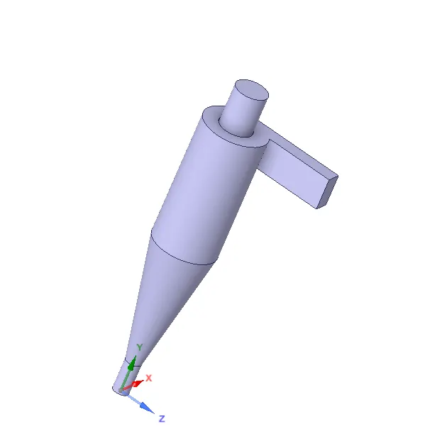
Save the file and close spaceclaim.
In the next stage, the geometry needs to be meshed. Right click on mesh and click methods and insert hex dominant so as to get uniform mesh. Next, we shall use two sizes of mesh( 8mm and 5mm) so as to determine whether any difference arise in the efficiency of the separators. Once done, the mesh looks something like this:
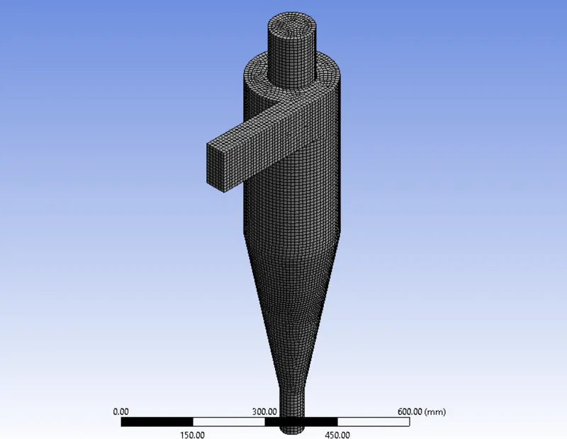
Provide named selections as:
Inlet
Outlet1(top)
Outlet2(bottom)
Update the mesh and exit meshing.
The next step involves setting up conditions in fluent solver.
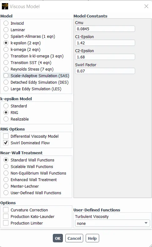
Viscous model-k-epsilon(RNG) with swirl dominated flow
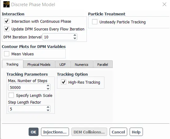
Discrete phase modeling (turned on)
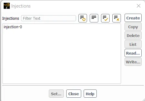
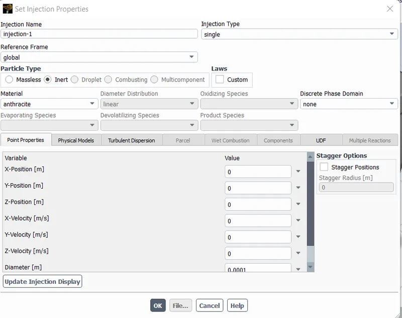
Injections-Create-surface-inlet and vary the particle size and inlet velocity respectively.
Once that is done, go to boundary conditions and change DPM of inlet, oultets as:
Inlet and wall:- Reflect
Outlet(Top):- Escape
Outlet(Bottom/dustbin) - Trap
Once done, initialise the solution and run for 500 iterations.
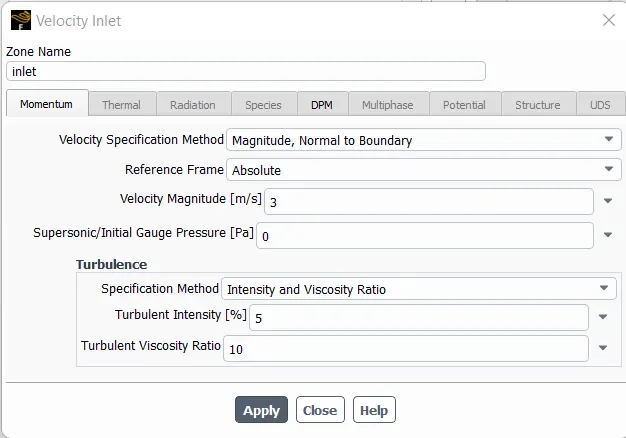
Once the solution is run, click on file->export->particle history data and save it to a file. Open CFD post and click on file->import->fluent particle data and import the file. The following are the results obtained from CFD-post.
Results:
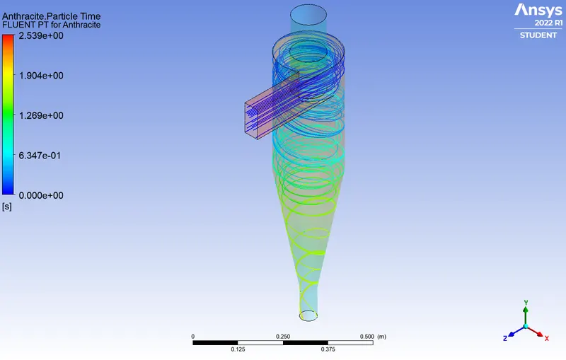
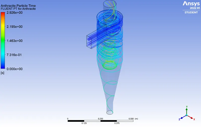
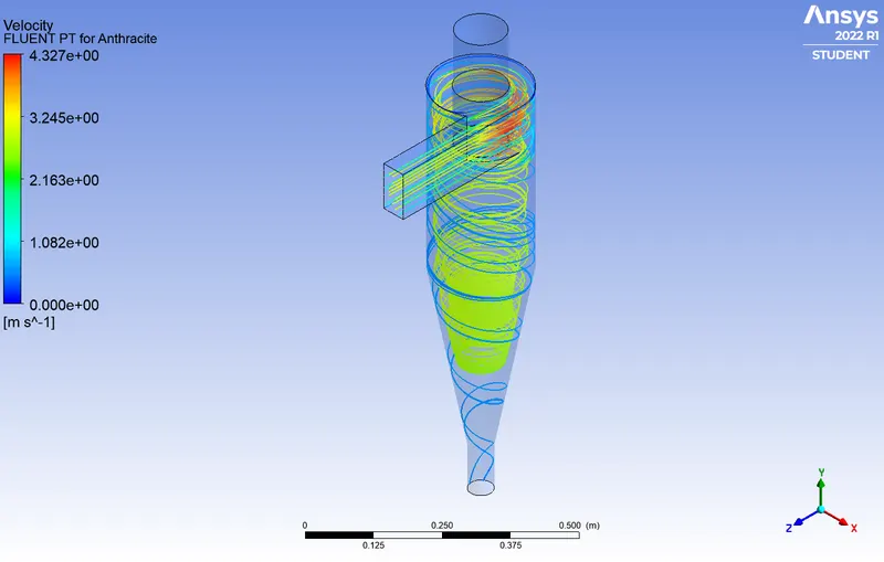
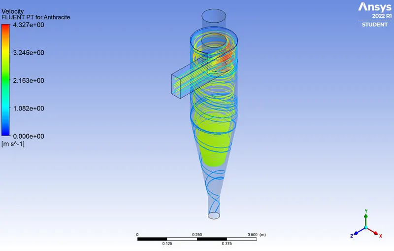
1. For constant velocity of 3m/s:
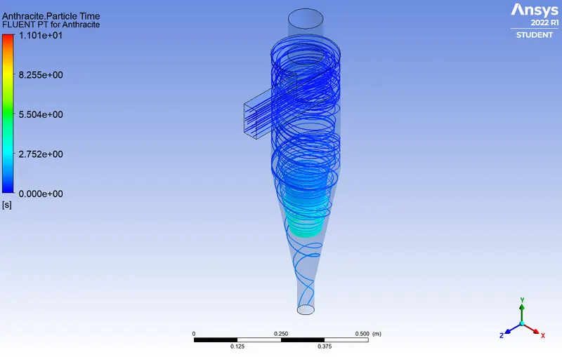
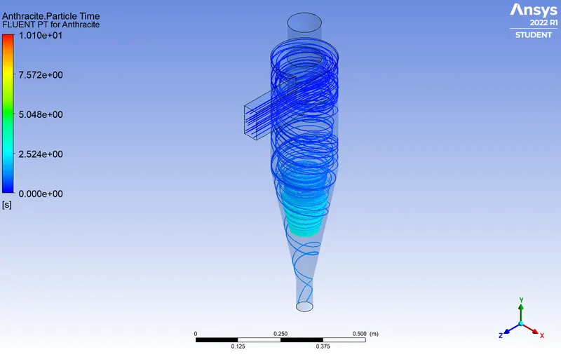
For cases with particle size of 1 `mum` and 3 `mum`, the mesh sizes are different as compared to particle sizes of 2 , 4 and 5 `mum`. This is done for comparative reasons so as to draw subtle conclusions whether meshing method changes the whole picture or not.
For mesh size of: 8 mm
Particle stay time
@ 1 `mum` @ 3`mum`
For mesh size of: 5mm
@ 2 `mum` @ 4`mum`
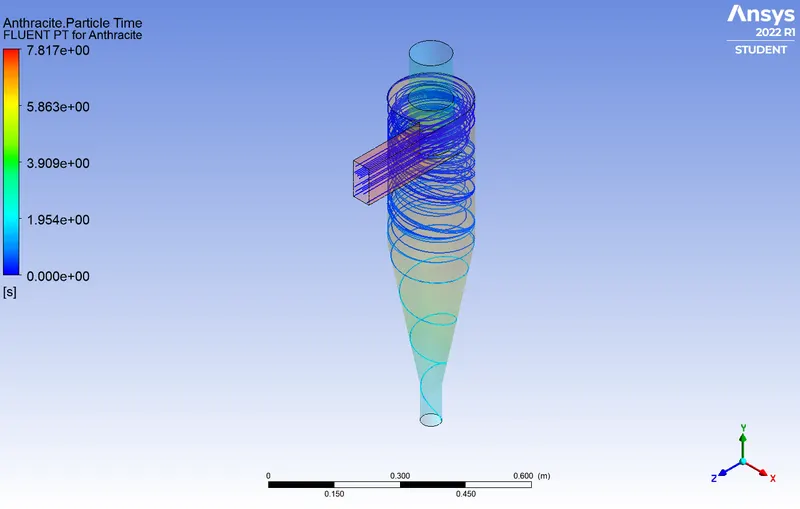
@ 5 `mum`
Velocity
@ 1 `mum` @ 3`mum`
@ 2 `mum` @ 4`mum`
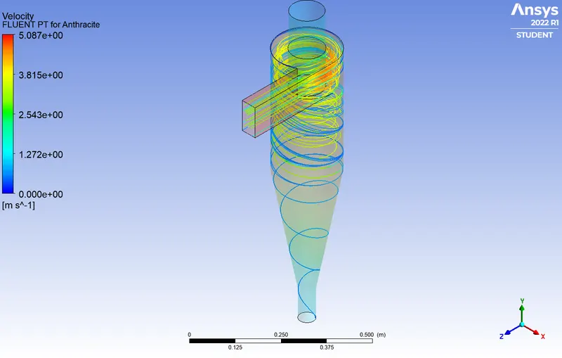
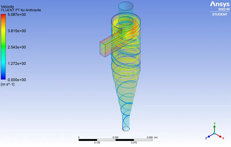
@ 5 `mum`
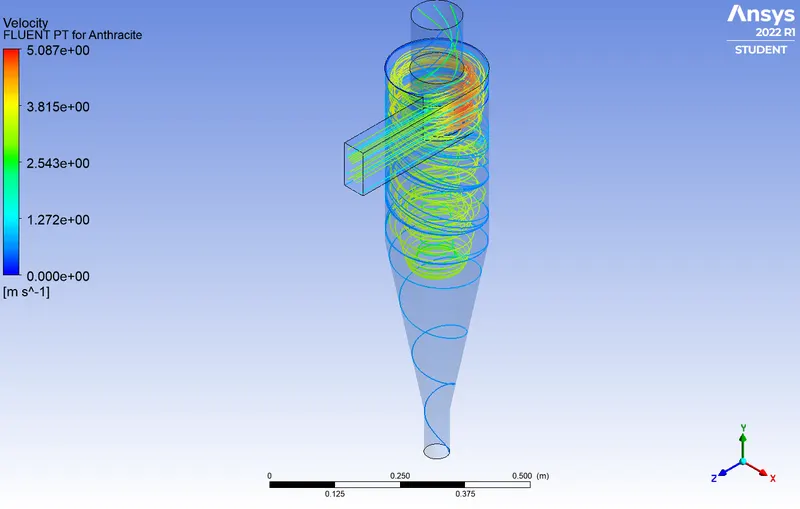
Pressure
@ 1 `mum` @ 3`mum`
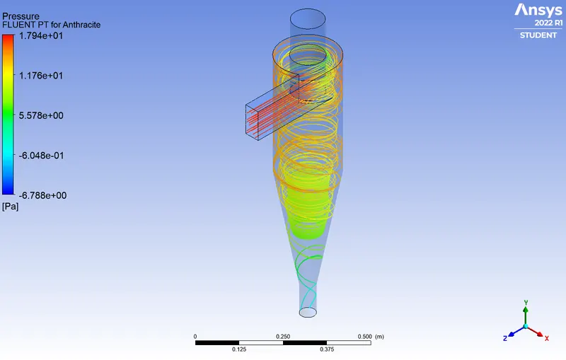
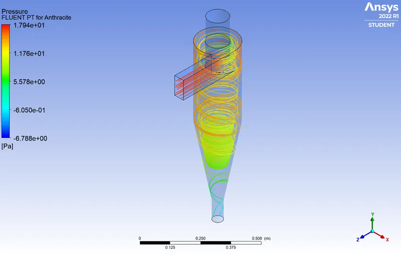
@ 2 `mum` @ 4`mum`
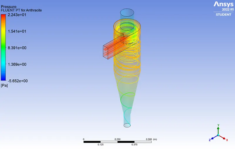
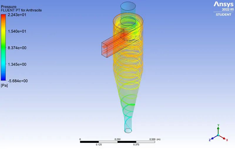
@ 5 `mum`
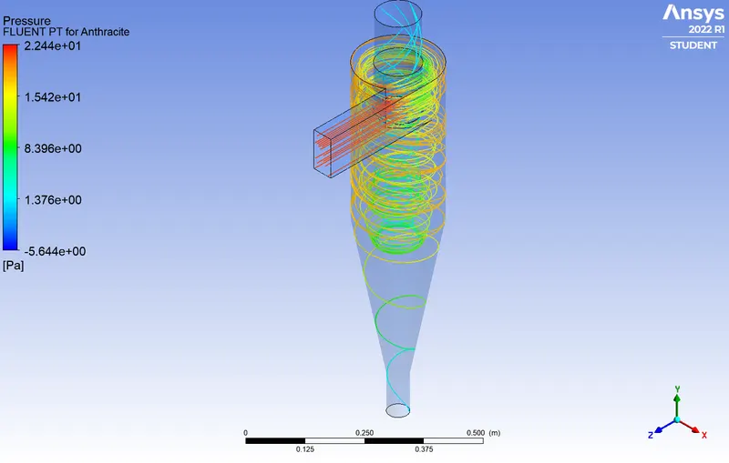
Vortex pattern
@ 1 `mum` @ 3`mum`
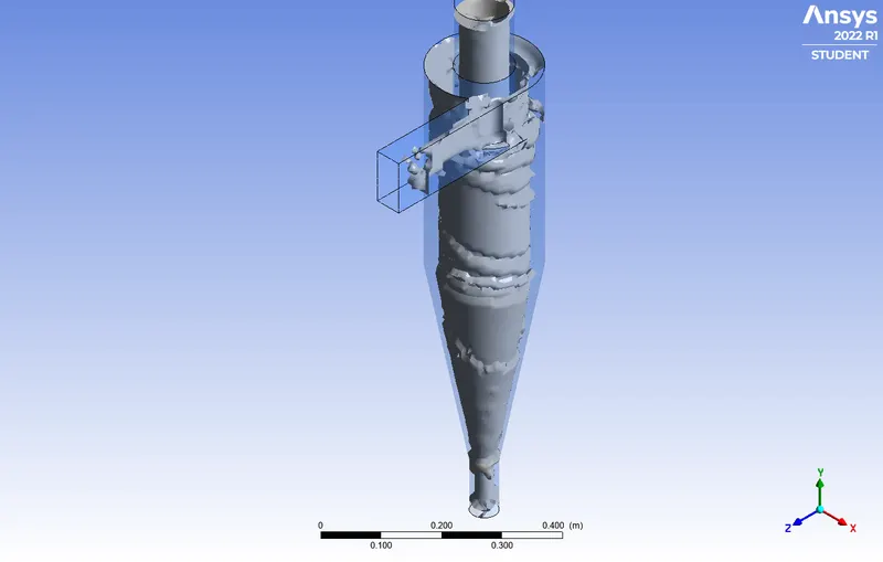
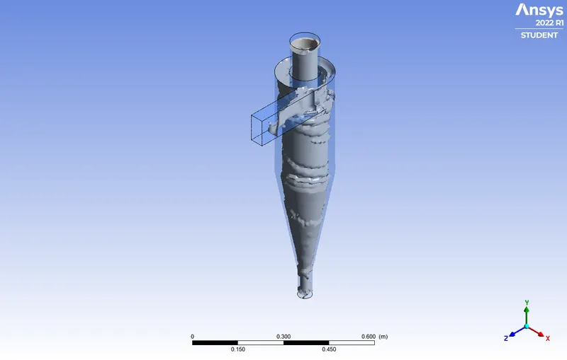
@ 2 `mum` @ 4`mum`
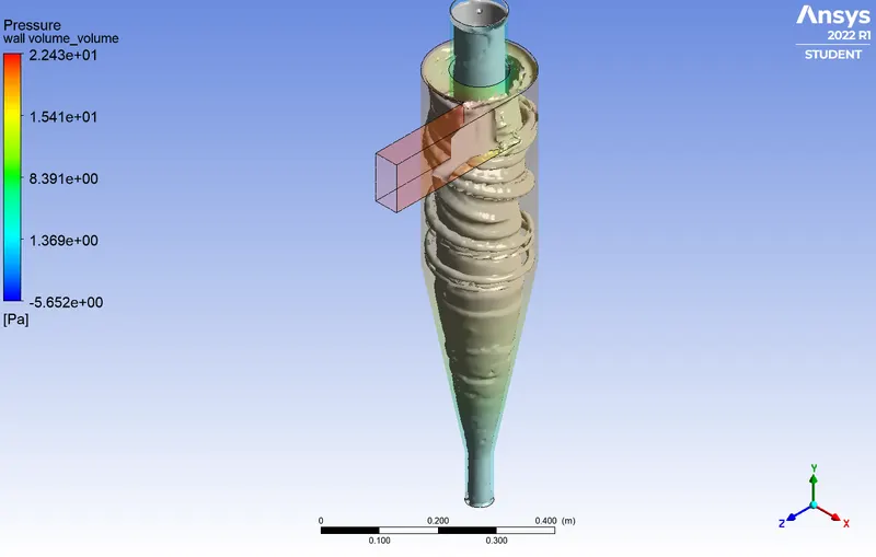
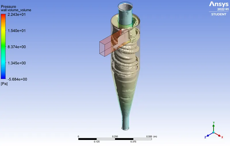
@ 5 `mum`
| Size of particulate (in µm) | No of particles tracked | No of particles escaped | No of particles trapped | Incomplete | Separation Efficiency |
| 1 | 78 | 11 | 52 | 15 | 0.666667 |
| 2 | 200 | 2 | 196 | 2 | 0.98 |
| 3 | 78 | 4 | 44 | 30 | 0.564103 |
| 4 | 200 | 0 | 200 | 0 | 1 |
| 5 | 200 | 54 | 146 | 0 | 0.73 |
Comparing size of particulates
Animation videos
For constant velocity of 3 m/s
For particle size of `1 mum`
https://drive.google.com/file/d/1VhE_rjCkDaYfQEstza1mUKB4Od4UL3W4/view?usp=sharing
For particle size of `2 mum`
https://drive.google.com/file/d/1wTxh-6-8N4ieaF6d6FcLLdvcHMvfjy8M/view?usp=sharing
For particle size of `3mum`
https://drive.google.com/file/d/1YVTYZPAS-2NtJcHaP_uuyXkt59IHH4o3/view?usp=sharing
For particle size of `4mum`
https://drive.google.com/file/d/1GvTewqISbSKv8HDvyxob8eQBELZLNlGn/view?usp=sharing
For particle size of `5mum`
https://drive.google.com/file/d/1GvTewqISbSKv8HDvyxob8eQBELZLNlGn/view?usp=sharing
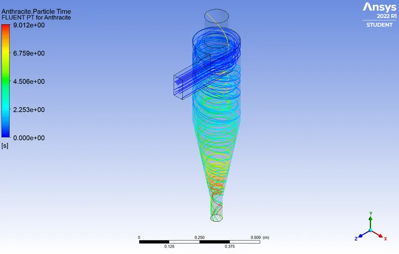
2. For constant particle size of 5`mum`
Particle stay time
@ 1 m/s @2m/s
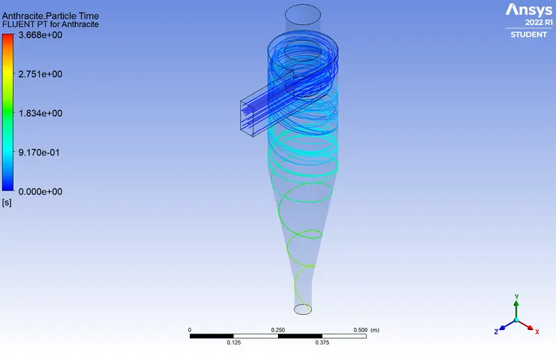
@3 m/s @4m/s
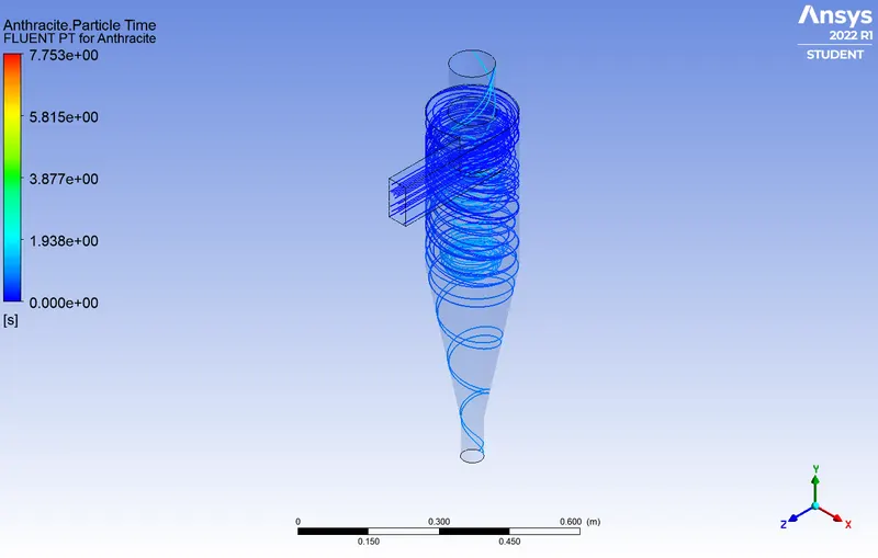
@5 m/s
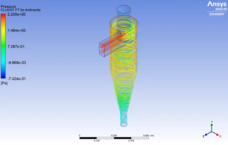
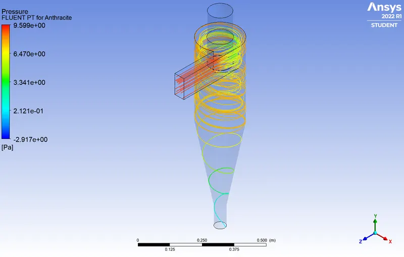
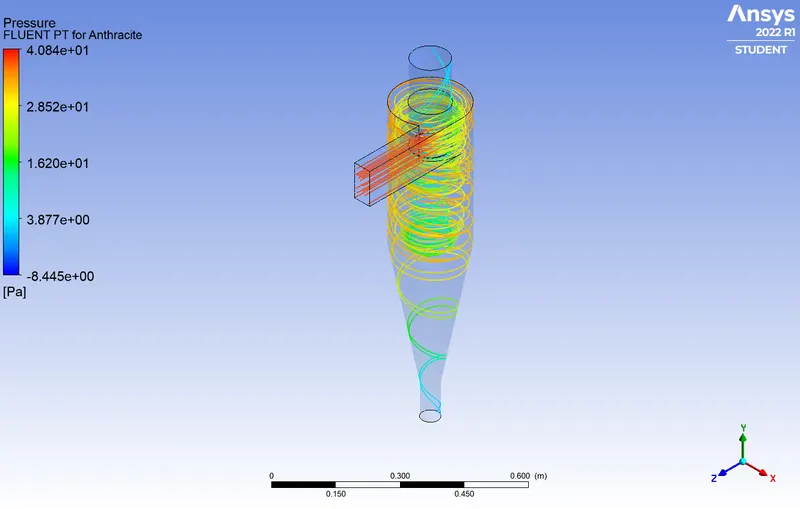
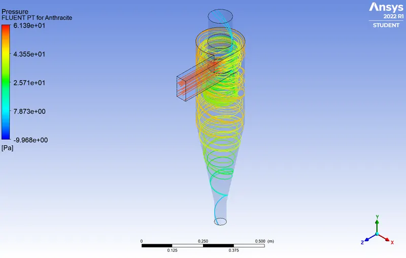
Pressure
@1 m/s @2m/s
@3 m/s @4 m/s
@5 m/s
Vortex:
@1 m/s @2m/s
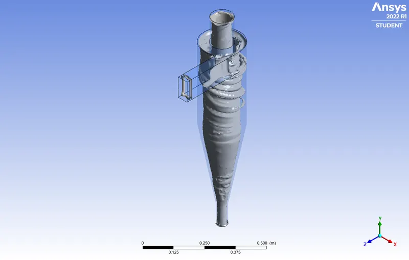
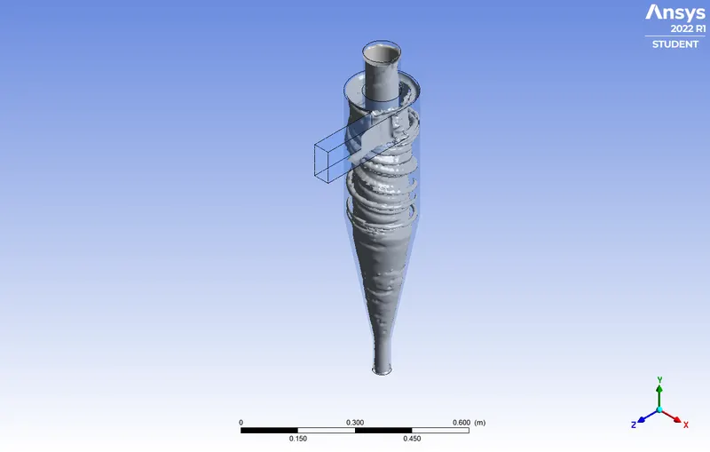
@3 m/s @4 m/s
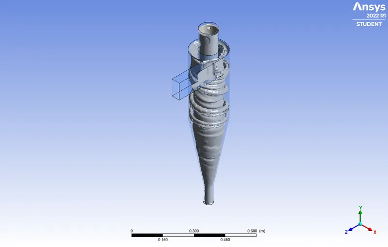
@5 m/s
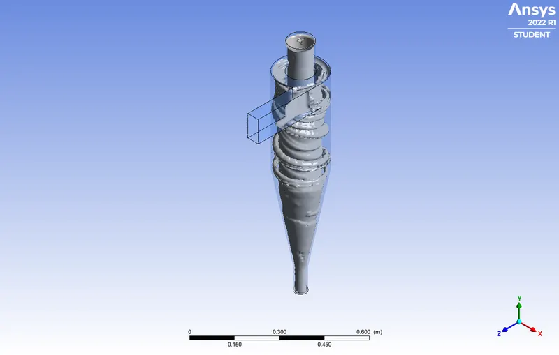
| Velocity(in m/s) | Mass flow rate | Pressure at inlet | Pressure at outlets | Pressure Drop | No of particles tracked | No of particles escaped | No of particles trapped | Incomplete | Separation Efficiency |
| 1 | 0.006125 | 4.4538 | 0.2657 | 4.1881 | 200 | 4 | 196 | 0 | 0.98 |
| 2 | 0.01225 | 9.1329 | 0.907943 | 8.224957 | 200 | 0 | 200 | 0 | 1 |
| 3 | 0.018375 | 17.2574 | 2.42209 | 14.83531 | 200 | 54 | 146 | 0 | 0.73 |
| 4 | 0.0245 | 38.6025 | 2.68684 | 35.91566 | 200 | 51 | 147 | 2 | 0.735 |
| 5 | 0.030625 | 57.8786 | 7.2835 | 50.5951 | 200 | 45 | 154 | 1 | 0.77 |
Velocity vs separation efficiency Velocity vs pressure drop
For constant particle size of 5`mum`
For velocity of 1 m/s
https://drive.google.com/file/d/1WEVepk5QE8mQuZRrA6bSiMgxrWJRLmvu/view?usp=sharing
For velocity of 2 m/s
https://drive.google.com/file/d/1beNb4fd5rI42OfQJR3ycyqfgQMV4Y4Bz/view?usp=sharing
For velocity of 3 m/s
https://drive.google.com/file/d/1YVTYZPAS-2NtJcHaP_uuyXkt59IHH4o3/view?usp=sharing
For velocity of 4 m/s
https://drive.google.com/file/d/1qjGD-y0kAyEWxg4UUFeDwcPCvSBtKybK/view?usp=sharing
For velocity of 5 m/s
https://drive.google.com/file/d/1GDIWuvuGmCsnOr-c1vGl5NM2ojzkqzux/view?usp=sharing
Conclusions:
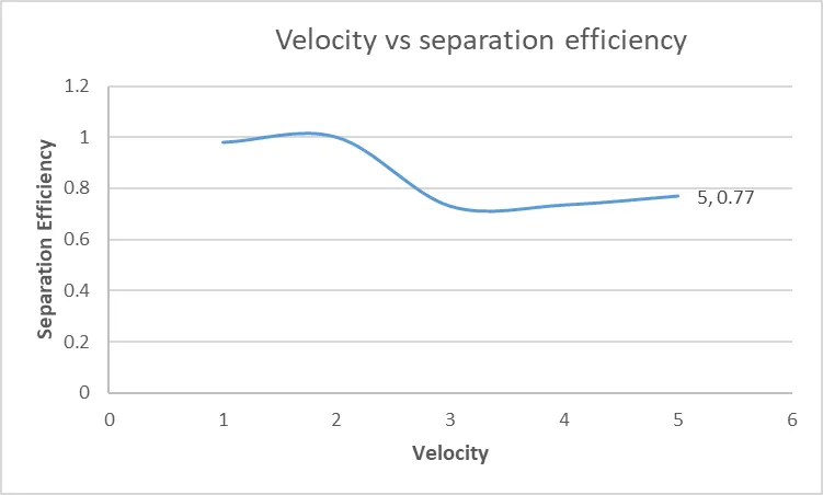
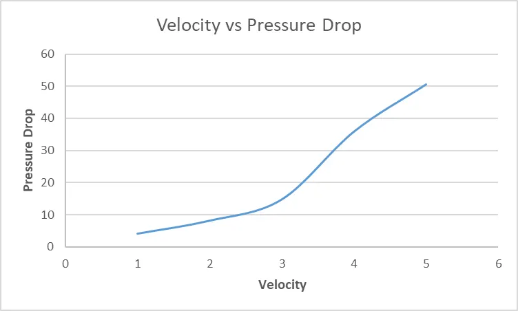
Thus the cyclone separator is simulated at different velocities and at different particle speeds. For this particular model, we can infer that the mesh size alters the number of particles escaping the separator and the number of particulates getting trapped in the settling chamber. Also we can infer that the pressure drop across the cyclone increases as the velocity of the dirty gas increases. And as the velocity of the dirty gas increases, the efficiency increases. Hence large particles can easily be separated by using this cyclone.