Week 8 - Simulation of a backward facing step in OpenFOAM
AIM
To simulate an incompressible laminar viscous flow through the backward facing step geometry and to perform a transient simulation. The test case should also be performed with 2 cases of grading factor and the results are enlisted.
THEORY AND PROCEDURE:
A laminar flow is one in which the reynolds number for that external flow is less than 300000. Reynolds number is defined as the ratio of inertial forces to that of viscous forces.
`Re=(rho*v*D)/mu` where `rho`->density of the fluid
`v`->velocity of the fluid
D-> characteristic length of the medium
`mu`-> dynamic viscosity of the medium.
This process involves setting up a geometry in openFOAM and meshing it using blockMesh and solving it.
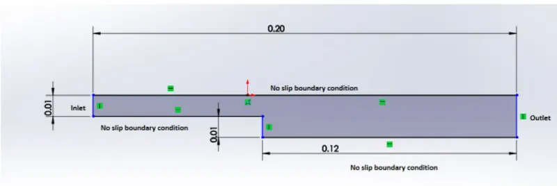
The geometry is 20 cm long and and there is a step halfway along the length of the geometry.
To construct this geometry, lets provide a thickness along the z-direction. 
The boundary names are specified at the domains.
To access the file, follow the given procedure.
In the command line, type tut. This will direct you to the tutorials folder in openFOAM.

- In the tutorials folder,type in ls. This will list down all folders in tutorials.
- Type in cd incompressible. This will direct you to the incompressible folder, from which you can select the desired solver to solve the backward step.
- Copy the folder from the tutorial folder to the run folder,where we will make changes and execute the program.
- Once the folder is copied into the run folder, sufficient changes are made to the existing files so as to achieve the desired results.
Description of files inside the folder
-->Preprocessing
Cases are setup in OpenFOAM by editing case files. Users should select an editor of choice with which to do this, such as emacs, vi, gedit, nedit, etc. Editing files is possible in Open-FOAM because the I/O uses a dictionary format with keywords that convey sufficient meaning to be understood by the users.
-->Meshing
OpenFOAM always operates in a 3 dimensional Cartesian coordinate system and all geometries are generated in 3 dimensions. OpenFOAM solves the case in 3 dimensions by default but can be instructed to solve in 2 dimensions by specifying a ‘special’ empty boundary condition on boundaries normal to the (3rd) dimension for which no solution is required. The domain consists of 0.2 m length domain with a step at halfway along the length of the domain.
| 2 | 3 |
| 1 | 4 |
| 5 |
Consider a domain divided into 5 blocks.
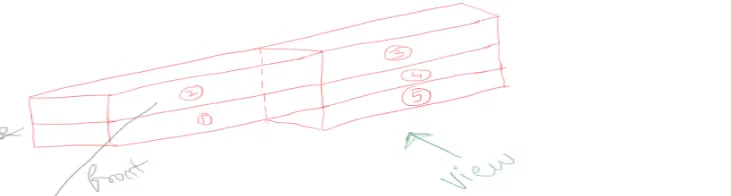
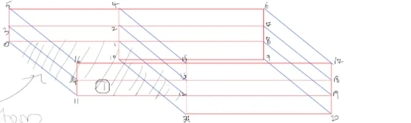
Since the flow velocity is assumed to be constant along z-direction,we only consider blocks along the 2D case. SInce a block is a 3D entity, there will be 8 vertices which are marked as shown.
The back face encloses the vertex nos 0 1 10 9 6 4 5 as a whole. Inside the blockMeshDict file, the coordinates of the vertices need to be specified first,followed by the faces.
Assuming that vertex 0 is the origin with entries(0,0,0). The other vertices can be plotted as such.
In the next step, the blocks needed to be specified. The type of mesh used is hexahedral. Inside the hex command, we have to specify vertices. The order of specification is to specify the vertices in the backface and frontface in counterclockwise direction. Next to the vertex nos, we define the number of divisions spaced along the co-ordinate axes. The simpleGrading command is used to specify whether a mesh is coarse or finer by defining expansion ratio which is the ratio of the width of the end cell to that of the start cell. Once the blocks are specified, the boundaries like the inlet and outlet are specified. Note that for specifying the boundary vertex, the back face is specified in the clockwise direction and the front face is specified in the counteclockwise direction.
A mesh of grading factor 1 and grading factor 0.2 is used as the two cases. The blockmesh is used to generate the mesh using the file blockMeshDict
blockMesh
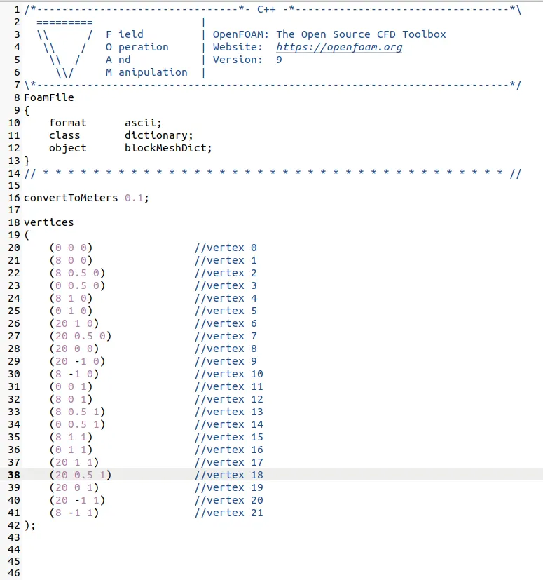
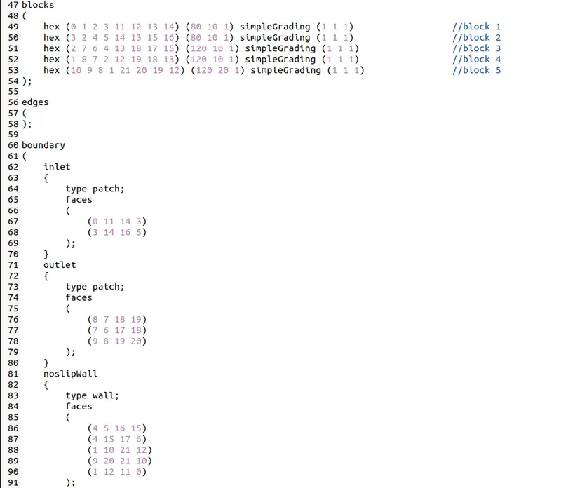
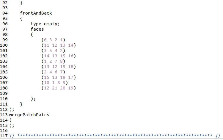
The file first contains header information in the form of a banner (lines 1-7), then file information contained in a FoamFile sub-dictionary, delimited by curly braces ({...}). For the remainder of the manual: For the sake of clarity and to save space, file headers, including the banner and FoamFile sub-dictionary, will be removed from verbatim quoting of case files. The file first specifies coordinates of the block vertices; it then defines the blocks (here, only 1) from the vertex labels and the number of cells within it; and finally, it defines the boundary patches.
The mesh is generated by running blockMesh on this blockMeshDict file. From within the case directory, this is done, simply by typing in the terminal: blockMesh
The running status of blockMesh is reported in the terminal window. Any mistakes in the blockMeshDict file are picked up by blockMesh and the resulting error message directs the user to the line in the file where the problem occurred. There should be no error messages at this stage.
-->Boundary and initial conditions
Once the mesh generation is complete, the user can look at this initial fields set up for this case. The case is set up to start at time t = 0 s, so the initial field data is stored in a 0 sub-directory of the cavity directory. The 0 sub-directory contains 2 files, p and U, one for each of the pressure (p) and velocity (U) fields whose initial values and boundary conditions must be set.
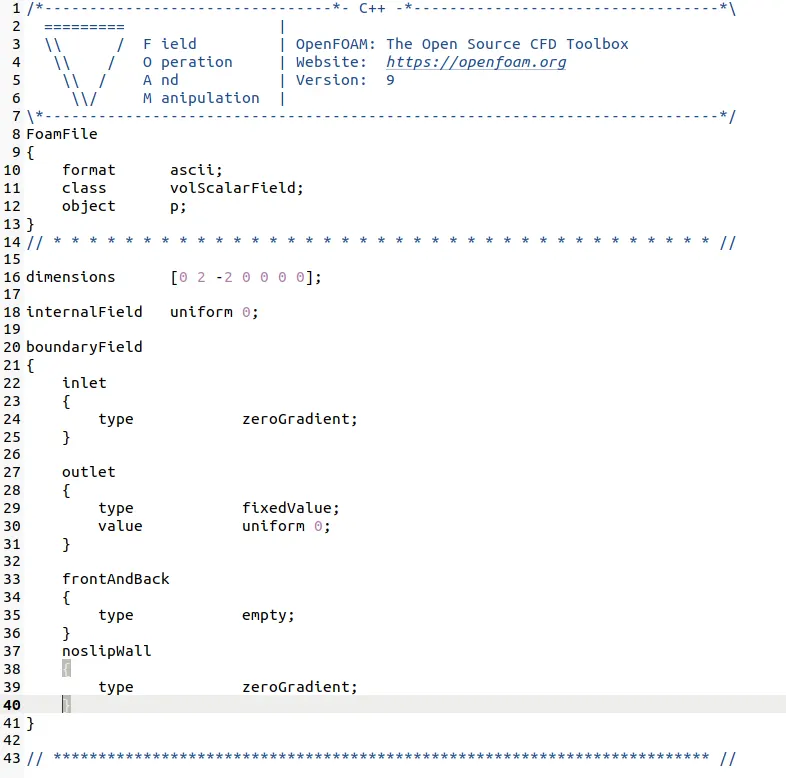
Pressure file:
Velocity file:
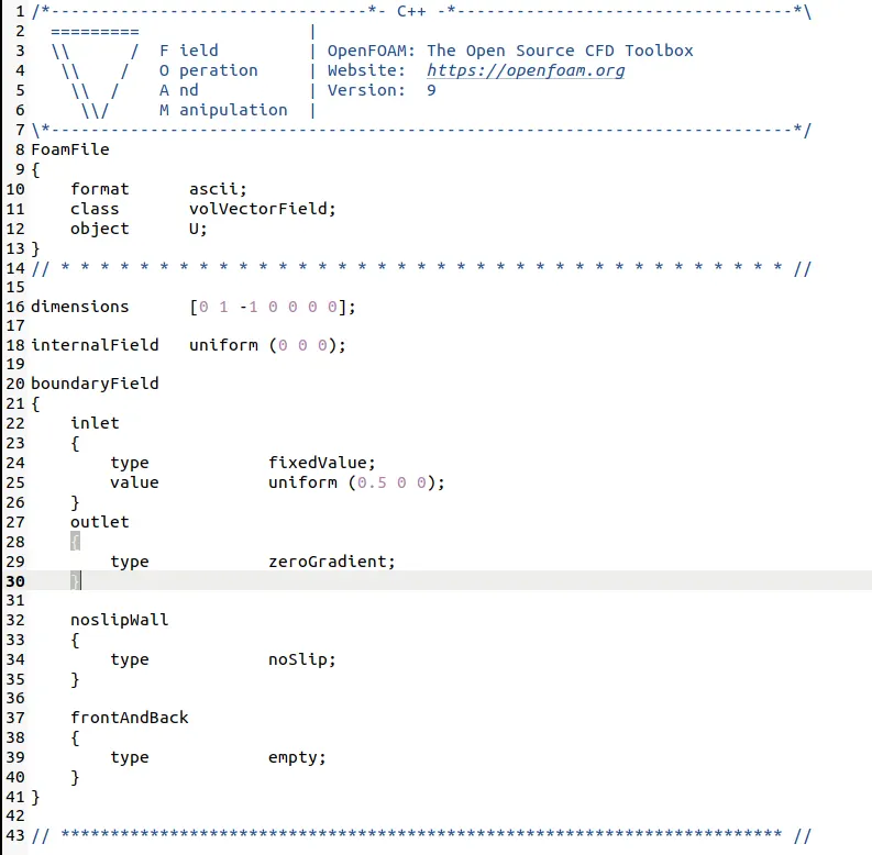
There are 3 principal entries in field data files:
dimensions -->specifies the dimensions of the field, here kinematic pressure, i.e. `m^2/s^2`
internalField -->the internal field data which can be uniform, described by a single value or nonuniform, where all the values of the field must be specified
boundaryField -->the boundary field data that includes boundary conditions and data for all the boundary patches
For the above case, the boundary consists of noslip wall.
As walls, both are given a zeroGradient boundary condition for p, meaning “the normal gradient of pressure is zero”. The frontAndBack patch represents the front and back planes of the 2D case and therefore must be set as empty. In this case, as in most we encounter, the initial fields are set to be uniform. Here the pressure is kinematic, and as an incompressible case, its absolute value is not relevant, so is set to uniform 0 for convenience. The boundary field for velocity requires the same boundary condition for the frontAndBack patch.
Physical Properties
The physical properties for the case are stored in dictionary files in the constant directory. For an icoFoam case, the only property that must be specified is the kinematic viscosity which is stored from the transportProperties dictionary. The user can check that the kinematic viscosity is set correctly by opening the transportProperties dictionary to view/edit its entries. The keyword for kinematic viscosity is `nu`. Assume the velocity as 0.5 m/s
Control
Input data relating to the control of time and reading and writing of the solution data are read in from the controlDict dictionary. The user should view this file; as a case control file, it is located in the system directory.The start/stop times and the time step for the run must be set. OpenFOAM offers great flexibility with time control.
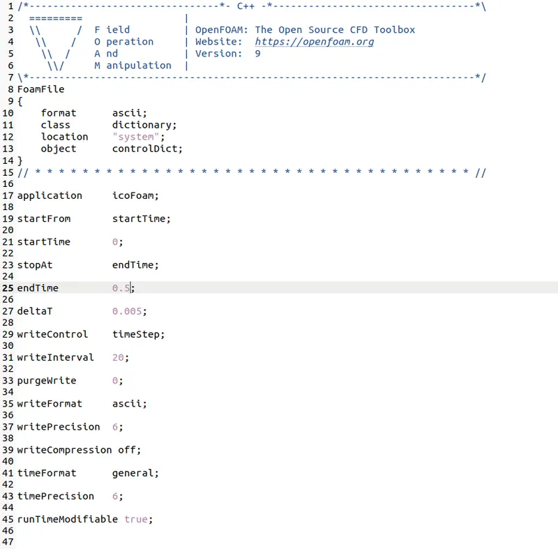
Now we need to set the time step, represented by the keyword `Deltat`. To achieve temporal accuracy and numerical stability when running icoFoam, a Courant number of less than 1 is required.
Courant no is defined as C=`(Deltat .U)/(Deltax)`
-->Running an application
openFOAM applications can be run either in the foreground or in the background. We will run icoFoam in the command line. The progress of the job is written to the terminal window. It tells the user the current time, maximum Courant number, initial and final residuals for all field.
-->Post-Processing
As soon as results are written to time directories, they can be viewed using paraFoam. Return to the paraFoam window and select the Properties panel for the cavity.OpenFOAM case module. If the correct window panels for the case module do not seem to be present at any time, please ensure that: cavity.OpenFOAM is highlighted in blue; eye button alongside it is switched on to show the graphics are enabled. To prepare paraFoam to display the data of interest, we must first load the data at the required run time of 0.5 s. If the case was run while ParaView was open, the output data in time directories will not be automatically loaded within ParaView. To load the data the user should uncheck Cache Mesh and click Refresh Times at the top Properties window (scroll up the panel if necessary). When The time data will be loaded into ParaView. In order to view the solution at t = 0.5 s, the user can use the VCR Controls or Current Time Controls to change the current time to 0.5.
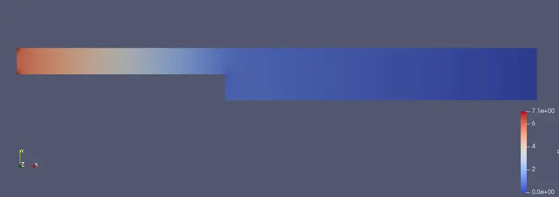
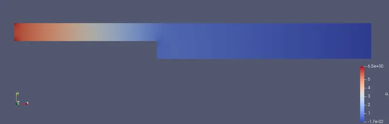
Pressure contour in the step with grading factor 1
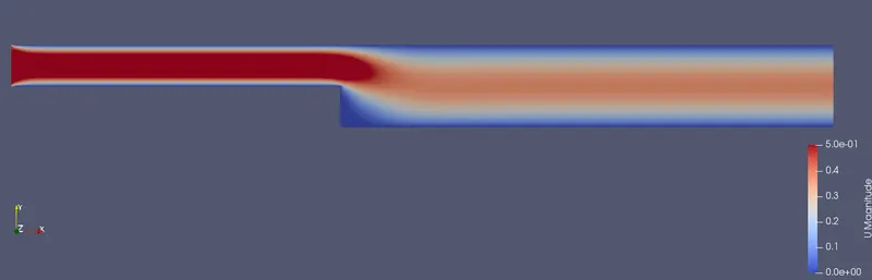
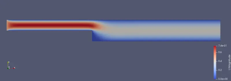
Velocity contour in the step with grading factor 1
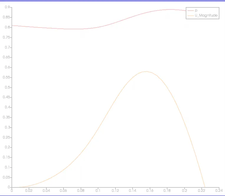
Velocity profile at a distance of 0.085 m from the inlet.
Meshing with grading factor of 0.2

Blockmesh file with 0.2 grading file
The only change neededto be made in the blockmesh file is that in the blocks heading by changing the grading factor appropriately.

Pressure contour in the step with grading factor 0.2
Velocity contour in the step with grading factor 0.2
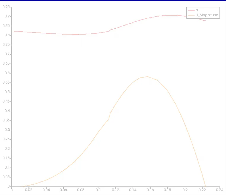
Comparing the above two graphs, we can infer that the profile is sharp for fine meshing with grading factor of 0.2. Hence grading factor is important in CFD where we needed to get accurate results.