Curve fitting comand
Curve fitting
what is curve fit ?
Curve fitting is the mathematical process in which we design the curve to fit the given data sets to a maximum extent. Here, we find the specific solution connecting the dependent and the independent variables for the provided data. The fitting should be as accurate as possible for the input data. The advantage of curve fitting is that it helps in optimizing the models to perform better.
the line passing through the circles is our curve .
the circles are the data set of any given values.
how to choose best fit.
-
The sum of squares due to error (SSE)
-
R-square
-
Adjusted R-square
-
Root mean squared error (RMSE)
formulas to find best fit
I=INDEPENDENT VARIABLE
M=MEAN (CP)
I=1
SSE=SUM ((CP-PREDICTED_CP) 2)
SSR=SUM ((PREDICTED_CP-M) 2)
SST=SSE+SSR
R2=SSR/SST
ADJUSTED R2 =1-(((1-R2)*(LENGTH (CP)-1))/ (LENGTH (CP)-I-1))
RMSE= SQRT (SSE/LENGTH (CP))
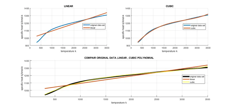
code to fit a linear and cubic polynomial for the Cp data.
clear all
close all
clc

%preparing the data
cp_data=load("data");
temperature=cp_data(:,1);
cp=cp_data(:,2);

% curve fit a linear polynomial for the Cp data.(with 1 degree)
%cp= ax+b
co_effs_1=polyfit(temperature,cp,1)
predicted_cp_1=polyval(co_effs_1,temperature);

% curve fit a cubic polynomial for the Cp data.(with 3 degree)
%cp= ax^3+bx^2+cx+d
co_effs_2=polyfit(temperature,cp,3)
predicted_cp_2=polyval(co_effs_2,temperature);

% COMPAIR OF ORIGINAL DATA AND LINEAR POLYNOMIAL
subplot(2,2,1)
hold on
plot(temperature,cp,LineWidth=3);
plot(temperature,predicted_cp_1,LineWidth=3)
xlabel("temperature {k}");
ylabel("specific heat {kj/kmol-k}");
legend("original data set",'linear')
title("LINEAR")
grid on

% COMPAIR OF ORIGINAL DATA AND CUBIC POLYNOMIAL
subplot(2,2,2)
hold on
plot(temperature,cp,LineWidth=3);
plot(temperature,predicted_cp_2,LineWidth=3)
xlabel("temperature {k}");
ylabel("specific heat {kj/kmol-k}");
legend("original data set","cubic")
title("CUBIC")
grid on

% COMPAIR OF ORIGINAL DATA ,LINEAR , CUBIC POLYNOMIAL
subplot(2,2,[3,4])
hold on
plot(temperature,cp,LineWidth=5,Color="k");
plot(temperature,predicted_cp_1,LineWidth=3)
plot(temperature,predicted_cp_2,LineWidth=2,Color="y")
xlabel("temperature {k}");
ylabel("specific heat {kj/kmol-k}");
legend("original data set","linear","cubic")
title("COMPAIR ORIGINAL DATA ,LINEAR , CUBIC POLYNOMIAL")
grid on

% CALCULATING GOODNESS FACTOR.

% calculating r_square andadjusted r_square forlinear
%i=independent variable
m=mean(cp)
i=1
sse_linear=sum((cp-predicted_cp_1).^2);
ssr_linear=sum((predicted_cp_1-m).^2);
sst_linear=sse_linear+ssr_linear;
r_square_linear=ssr_linear/sst_linear;
adjusted_r_square_linear=1-(((1-r_square_linear)*(length(cp)-1))/(length(cp)-i-1));
rmse_linear= sqrt(sse_linear/length(cp));


% calculating r_square  and adjusted r_square for cubic
sse_cubic=sum((cp-predicted_cp_2).^2);
ssr_cubic=sum((predicted_cp_2-m).^2);
sst_cubic=sse_cubic+ssr_cubic;
r_square_cubic=ssr_cubic/sst_cubic;
adjusted_r_square_cubic=1-(((1-r_square_cubic)*(length(cp)-1))/(length(cp)-i-1));
rmse_cubic= sqrt(sse_cubic/length(cp));


%error
name_of_error=["sse";"r_square";"adjust_r";"rmse"];
linear_error=[sse_linear;r_square_linear;adjusted_r_square_linear;rmse_linear];
cubic_error=[sse_cubic;r_square_cubic;adjusted_r_square_cubic;rmse_cubic];
goodness_parameter=table(linear_error,cubic_error,name_of_error)
all graph using subplot comand
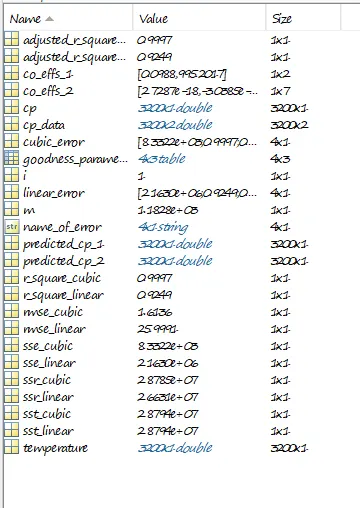
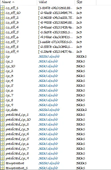
workspace
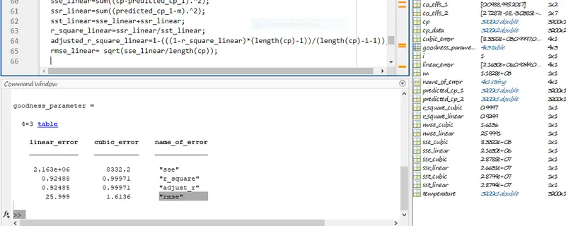
explanation
step1: preparing the input data as showning videos.
step2: prividing temperatuer and cp column
step3:using polyfit comand for calculating a and b where x= temperature
step4: using polyval comand to predict the values of cp
step5:using subplot to plot 3 graph to plot into single display.
step6:using of hold on command to plot both original plots and curvefit plot in 1 graph
step7: calculating goodness factor for which need to give the formulas and values of {sse,ssr,sst,r_square,adjust rsquare,rmse}
{{make sure of using element wise oprator (.)in sse and ssr because values are in metrix form}}
step8:showing error in the form of table.
code to show splitwise method.
clear all
close all
clc

%preparing the data
cp_data=load("data");
temperature=cp_data(:,1);
cp=cp_data(:,2);

% dividing data into 10 set for splitwise method.

temperature_1=cp_data(1:320,1);
cp_1=cp_data(1:320,2);

temperature_2=cp_data(321:640,1);
cp_2=cp_data(321:640,2);

temperature_3=cp_data(641:960,1);
cp_3=cp_data(641:960,2);

temperature_4=cp_data(961:1280,1);
cp_4=cp_data(961:1280,2);

temperature_5=cp_data(1281:1600,1);
cp_5=cp_data(1281:1600,2);

temperature_6=cp_data(1601:1920,1);
cp_6=cp_data(1601:1920,2);

temperature_7=cp_data(1921:2240,1);
cp_7=cp_data(1921:2240,2);

temperature_8=cp_data(2241:2560,1);
cp_8=cp_data(2241:2560,2);

temperature_9=cp_data(2561:2880,1);
cp_9=cp_data(2561:2880,2);

temperature_10=cp_data(2881:3200,1);
cp_10=cp_data(2881:3200,2);


% curve fit  for the Cp data.(with 2 degree)
%cp= ax^2+bx+c
co_eff_1=polyfit(temperature_1,cp_1,2);
predicted_cp_1=polyval(co_eff_1,temperature_1);

co_eff_2=polyfit(temperature_2,cp_2,2);
predicted_cp_2=polyval(co_eff_2,temperature_2);

co_eff_3=polyfit(temperature_3,cp_3,2);
predicted_cp_3=polyval(co_eff_3,temperature_3);

co_eff_4=polyfit(temperature_4,cp_4,2);
predicted_cp_4=polyval(co_eff_4,temperature_4);

co_eff_5=polyfit(temperature_5,cp_5,2);
predicted_cp_5=polyval(co_eff_5,temperature_5);

co_eff_6=polyfit(temperature_6,cp_6,2);
predicted_cp_6=polyval(co_eff_6,temperature_6);

co_eff_7=polyfit(temperature_7,cp_7,2);
predicted_cp_7=polyval(co_eff_7,temperature_7);

co_eff_8=polyfit(temperature_8,cp_8,2);
predicted_cp_8=polyval(co_eff_8,temperature_8);

co_eff_9=polyfit(temperature_9,cp_9,2);
predicted_cp_9=polyval(co_eff_9,temperature_9);

co_eff_10=polyfit(temperature_10,cp_10,2);
predicted_cp_10=polyval(co_eff_10,temperature_10);

% plotting the curve fit
hold on
plot(temperature,cp,LineWidth=7,Color="k")
plot(temperature_1,predicted_cp_1,Color="w",LineWidth=2)
plot(temperature_2,predicted_cp_2,Color="w",LineWidth=2)
plot(temperature_3,predicted_cp_3,Color="w",LineWidth=2)
plot(temperature_4,predicted_cp_4,Color="w",LineWidth=2)
plot(temperature_5,predicted_cp_5,Color="w",LineWidth=2)
plot(temperature_6,predicted_cp_6,Color="w",LineWidth=2)
plot(temperature_7,predicted_cp_7,Color="w",LineWidth=2)
plot(temperature_8,predicted_cp_8,Color="w",LineWidth=2)
plot(temperature_9,predicted_cp_9,Color="w",LineWidth=2)
plot(temperature_10,predicted_cp_10,Color="w",LineWidth=2)
xlabel("temperature {k}");
ylabel("specific heat {kj/kmol-k}");
legend("original data set","split wise")
title("split wise")
grid on
out put plot of split wise curve fit.
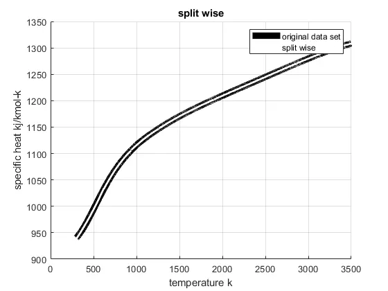
split wise method provides can provide the best fit with minium error.
explanation
step1:inserting the data
step 2 dividing data into 10 parts
step3:using polyfit comand for calculating a and b where x= temperature
step4: using polyval comand to predict the values of cp
[this step is repeated 10 times because the data is divide into 10 parts.
step5 using hold on comand to plot all curves on 1 graph
step6:plotting all 10 curves on one graph .
answer are written in my onw words no copy.
How to make a curve fit perfectly?
to make the fit perfectly using of inbuild app of curve fit . perfecttly fit means all points should be joined with the curve but this cannot be possibe there will be some of the points that are not into a curve .
How to get the best fit?
best fit can be get by using split wise oprator it is the best method to get best fit .if the value of r square is grater then 0.95 then the fit is to be known as best fit.
using of high degree polynomial can also be used but more possibility of getting error are there.
What could be done to improve the cubic fit?
best wyay is to do split wise method with cubic fit, in which we divides the input into multipal parts and make carve of it which minimes the error.
error that i had faced a lot whicle coding
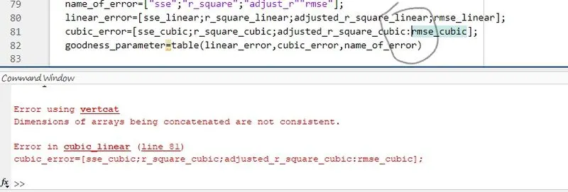
forgot to add (;)
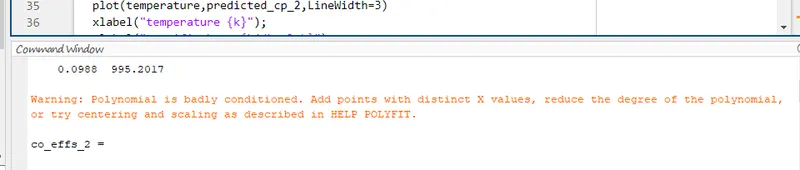
when ther is high order of polynomial
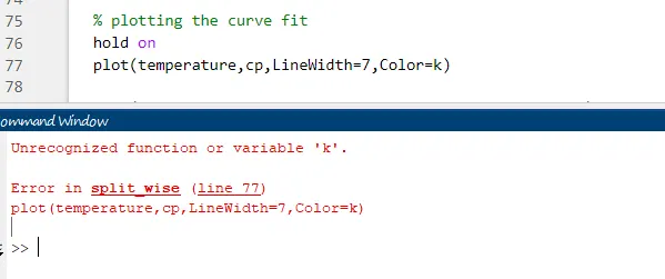
forgot to add "k"
refrence
https://skill-lync.com/student-projects/Curve-Fitting-and-criterion-to-choose-best-fit-41860
youtube.com/watch?v=9ikmTD0bpOc
thank you