Week 4.1 - Genetic Algorithm
Genetic Algorithm
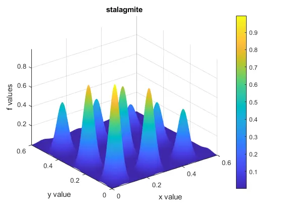
aim:- Write a code in MATLAB to optimise the stalagmite function and find the global maxima of the function.
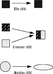
concept of ga is to solve non linear and non differentiable optimization problem by finding the global minimum to optimization problem( means the smallest overall value of a set, function, etc., over its entire range. It is impossible to construct an algorithm that will find a global minimum for an arbitrary function.) this is been done by copying the evolutionary biology technique. starting with an initial generation of candidates solutions that are tested against the objective function.then selection ,crossover and mutation. ga always minimize the function value.
 [evolutionary biology technique]
election
these are the values of first generation
parents 1= [1 0 1 0 0 1 1 0 0 0 ]
parents 2= [1 0 0 1 0 0 1 0 1 0 ]
cross over
due to perfoming well in previous generatio they have been selected for second generation and crossover is done and producinf child in which common similarity from parents is keep same.
parents 1= [1 0 1 0 0 1 1 0 0 0 ]
parents 2= [1 0 0 1 0 0 1 0 1 0 ]
child = [1 0 0 0 0 1 1 0 1 0 ]
mutation
in this we take a parent and mutation is done means modifing and creating a child from it.
parent = [1 0 1 0 0 1 1 0 0 0 ]
child = [0 1 0 1 0 1 0 0 0 1 ]
due to mutation avoide falling in local minima and it really helps them explore the solution space well.
example
what is the syntax for ga in MATLAB ?
x = ga(fun,nvars)
x = ga(fun,nvars,A,b)
x = ga(fun,nvars,A,b,Aeq,beq)
x = ga(fun,nvars,A,b,Aeq,beq,lb,ub)
x = ga(fun,nvars,A,b,Aeq,beq,lb,ub,nonlcon)
x = ga(fun,nvars,A,b,Aeq,beq,lb,ub,nonlcon,options)
x = ga(fun,nvars,A,b,Aeq,beq,lb,ub,nonlcon,intcon)
x = ga(fun,nvars,A,b,Aeq,beq,lb,ub,nonlcon,intcon,options)
x = ga(problem)
[x,fval] = ga(___)
[x,fval,exitflag,output] = ga(___)
[x,fval,exitflag,output,population,scores] = ga(___)
x = ga(fun,nvars) finds a local unconstrained minimum, x, to the objective function, fun. nvars is the dimension (number of design variables) of fun.
x = ga(fun,nvars,A,b) finds a local minimum x to fun, subject to the linear inequalities A*x ≤ b. ga evaluates the matrix product A*x as if x is transposed (A*x').
x = ga(fun,nvars,A,b,Aeq,beq) finds a local minimum x to fun, subject to the linear equalities Aeq*x = beq and A*x ≤ b. (Set A=[] and b=[] if no linear inequalities exist.) ga evaluates the matrix product Aeq*x as if x is transposed (Aeq*x').
x = ga(fun,nvars,A,b,Aeq,beq,lb,ub) defines a set of lower and upper bounds on the design variables, x, so that a solution is found in the range lb ≤ x ≤ ub. (Set Aeq=[] and beq=[] if no linear equalities exist.)
x = ga(fun,nvars,A,b,Aeq,beq,lb,ub,nonlcon) subjects the minimization to the constraints defined in nonlcon. The function nonlcon accepts x and returns vectors C and Ceq, representing the nonlinear inequalities and equalities respectively. ga minimizes the fun such that C(x) ≤ 0 and Ceq(x) = 0. (Set lb=[] and ub=[] if no bounds exist.)
x = ga(fun,nvars,A,b,Aeq,beq,lb,ub,nonlcon,options) minimizes with the default optimization parameters replaced by values in options. (Set nonlcon=[] if no nonlinear constraints exist.) Create options using optimoptions.
x = ga(fun,nvars,A,b,Aeq,beq,lb,ub,nonlcon,intcon) or x = ga(fun,nvars,A,b,Aeq,beq,lb,ub,nonlcon,intcon,options) requires that the variables listed in intcon take integer values.
x = ga(problem) finds the minimum for problem, a structure described in problem.
[x,fval] = ga(___), for any previous input arguments, also returns fval, the value of the fitness function at x.
[x,fval,exitflag,output] = ga(___) also returns exitflag, an integer identifying the reason the algorithm terminated, and output, a structure that contains output from each generation and other information about the performance of the algorithm.
[x,fval,exitflag,output,population,scores] = ga(___) also returns a matrix population, whose rows are the final population, and a vector scores, the scores of the final population.
where ga is an inbuild function by mathlab then providing the objective function then the dimensions.
in case we do not have the values of A,b,Aeq,beq,lb,ub,nonlcon,intcon,options we need to put [] in that space.
code to optimise the stalagmite function
clear all
close all
clc

%defining our search space
 x=linspace(0,0.6,150);
 y=linspace(0,0.6,150);
 num_cases=50;                                  % running ga 50 times

 %converting 2d plot of x and y which were in 1d
 [xx,yy]=meshgrid(x,y);

  for k=1:length(xx);                           % values of xx
     for j=1:length(yy);                        % values af yy
         input_vector(1)=xx(k,j);               %creating array  each values from xx
         input_vector(2)=yy(k,j);               %creating array  each values from yy
         f(k,j)=stalagmite(input_vector);       % function creates for stalagmite in figure
     end
 end

 figure(1)
surfc(xx,yy,-f)                                 % making graph figure from xx,yy,f values
shading("interp")                               % removing lines from the plot giving smooth look
xlabel("x value")
ylabel("y value")
zlabel("f values")
colorbar
title('stalagmite')

%study 1 satistical behaviour
  tic                                            % time start
 for i=1:num_cases;
     [inputs,fopt(i)]=ga(@stalagmite,2);
     xopt(i)=inputs(1);
     yopt(i)=inputs(2);
 end
study_1_time=toc                                      % end time stored in study_1

 figure(2)
 subplot(2,1,1)                                       % to attach two graph in one screen.
 hold on
surfc(x,y,f)
shading interp
% plotting the optimum points
plot3(xopt,yopt,fopt,Marker='o',MarkerSize=5,MarkerFaceColor='r')
title('unbounded inputs')
xlabel("x value")
ylabel("y value")
subplot(2,1,2)
plot(fopt)
xlabel("iteration")
ylabel("function minimum")
tic
% study 2-statistical behavior -with upper and lower bonds
 for i=1:num_cases;
     [inputs,fopt(i)]=ga(@stalagmite,2,[],[],[],[],[0;0],[0.6;0.6]);  % giving upper and lower boundry  for ga
     xopt(i)=inputs(1);
     yopt(i)=inputs(2);
 end
study_2_time=toc


 figure(3)
subplot(2,1,1)
hold on
surfc(x,y,f)
shading interp
plot3(xopt,yopt,fopt,Marker='o',MarkerSize=5,MarkerFaceColor='r')
title('bounded inputs')
xlabel("x value")
ylabel("y value")
subplot(2,1,2)
plot(fopt)
xlabel("iteration")
ylabel("function minimum")

% study 3 increasing ga iterations
options =optimoptions("ga");
options=optimoptions(options,PopulationSize=400);           % changing initial population size so that we can get global minima
% instade of global local minima
tic
for i=1:num_cases;
     [inputs,fopt(i)]=ga(@stalagmite,2,[],[],[],[],[0;0],[0.6;0.6],[],[],options);
     xopt(i)=inputs(1);
     yopt(i)=inputs(2);
 end
study_3_time=toc


 figure(4)
subplot(2,1,1)
hold on
surfc(x,y,f)
shading interp
plot3(xopt,yopt,fopt,Marker='o',MarkerSize=5,MarkerFaceColor='r')
title('bounded inputs')
xlabel("x value")
ylabel("y value")
subplot(2,1,2)
plot(fopt)
xlabel("iteration")
ylabel("function minimum")

% creatin table for time
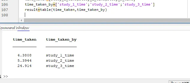
time_taken=[study_1_time;study_2_time;study_3_time]
time_taken_by=['study_1_time';'study_2_time';'study_3_time']
result=table(time_taken,time_taken_by)
function codes which is created
function f=stalagmite(input_vector)
x= input_vector(1);
y= input_vector(2);
f1=(sin((5.1*pi*x)+0.5)).^6;
f2=exp((-4*log(2))*(((x-0.0667).^2)/0.64));
f3=(sin((5.1*pi*y)+0.5)).^6;
f4=exp((-4*log(2))*((y-0.0667).^2)/0.64);
f=-(f1.*f2.*f3.*f4);
end
output plots
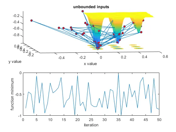
study 1 plot
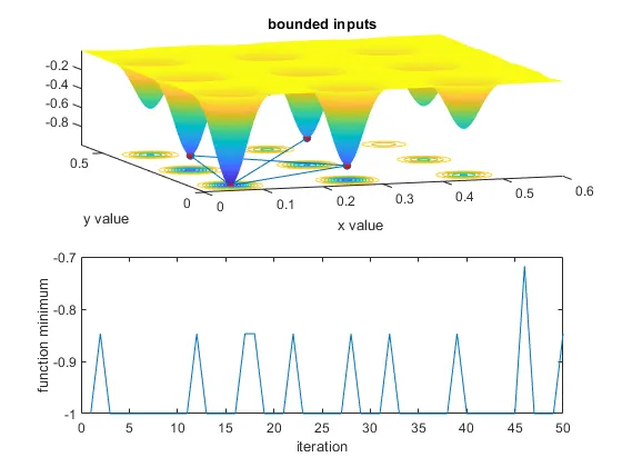
study 2 plot
study 3 plot
time take by each graph
explanation of the code
first providing x values and y values using linspace command which are 1 diamention values.
then converting x and y values into xx and yy values using meshgrid command which are 2 dimention values
then using numcase this is to run ga 50 time.
creating the loop which will provide a stalagmite design in the graph
first loop take the values of xx and second loop take the values of yy and will be provided to input vectors
stalagmite is the function which is been created
then using surfc command to plot xx,yy -f values {-f is used to make the stalagmite figure not to be in inverse direction}
shading("interp") comand is used to make the plot look smooth an remove grid from it.
providing x label, ylabel,z label,title and colorbar.
now ,
study 1
where we are using ga command and providing stalagmit function then no in inputes vlues which are xopt and yopt
and running it for 50 time using of tic and toc command to not how much time does itake.
using subplot to plot two plot in figure
first plot is plot3 comand which shows stalagmit figure with random points
second plot is fopt which shows the values of -1 to 1 because boundries were not defined . and so study 1 gives n number of values.
study 2
running for 50 time using of tic and toc command to not how much time does itake.
in ga providing [] which are blank space , then providing upper and lower bondries we provided this because ga function was picking random valuse which was not defined and now you can see study 2 graph with very less points which are local maxima.
study 3
running for 50 time using of tic and toc command to not how much time does itake.
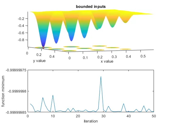
giving options=optimoptions(options,PopulationSize=400) means changing initial population size so that we can get global minima instade of global local minima as shown in study 2.
now every time well run the code will get the same values and
study 3 figure shows the value of -0.99999 whic opposit of the global maxima thats means the global maxima will be 0.9999
explanation of function
x and y are the input vector and f1,f2,f3,f4 are the formulas
f=-(f1.*f2.*f3.*f4) puting (-) because ga always provide the global minima and we need to find he globlal maxima to we use the (-) sign so the the answer wll be reverse and we can get global maxima instade of global minima
errors got in the program
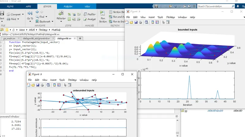
this error was due to not putting - sign in function and it took 3 days me to understand
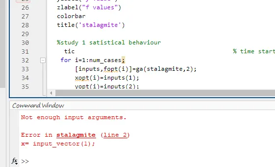
error 2
due to not putting @ before stalagmite because ga is a function and stalagmite in another function sowhen using function under another function need to add @.
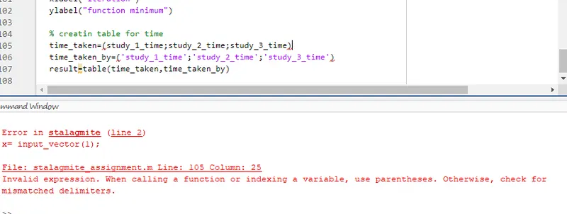
error3
due to not providing this bracket [] because this brackes are used for a matrix opner
referance
https://in.mathworks.com/help/gads/ga.html
https://in.mathworks.com/discovery/genetic-algorithm.html
https://in.mathworks.com/videos/what-is-a-genetic-algorithm-100904.html
thank you