Week 3 - Solving second order ODEs
Solving second order ODEs
aim:write a program that solves the following ODE. This ODE represents the equation of motion of a simple pendulum with damping
what is an ODE?
The Ordinary Differential Equation (ODE) solvers in MATLAB solve initial value problems with a variety of properties. The solvers can work on stiff or nonstiff problems, problems with a mass matrix, differential algebraic equations (DAEs), or fully implicit problems. For more information, see choose and solve.
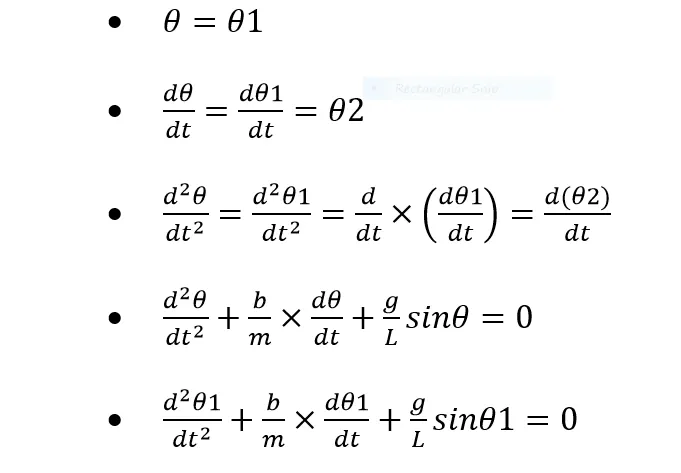
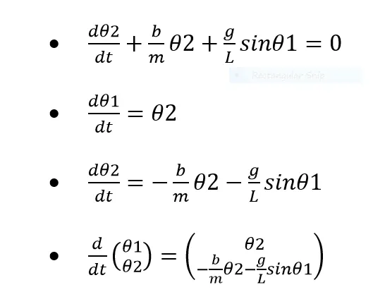
to solve any ODE first we need to convert it into first order ODE.
this equatin is of second order ODE so first we need to convert it two first order ODE.which will give us two values displacement and velocity in oue question.
In the above equation,
g = gravity in m/s2,
L = length of the pendulum in m,
m = mass of the ball in kg,
b=damping coefficient.
use,
L=1 metre,
m=1 kg,
b=0.05.
g=9.81 m/s2.
CONVERION OF ODE TO 2 FIRST ORDER ODE
PREPARING FUNCTION
function  [dtheta_dt]= ode_func(t,theta,b,g,p,m)
theta1=theta(1)
theta2=theta(2)
dtheta1_dt=theta2;
dtheta2_dt=-(b/m)*theta2-(g/p)*sin(theta1);
dtheta_dt= [dtheta1_dt;dtheta2_dt]
end
the function has been explaned above that how we convert second order odes into two first order ODE.
for simple pendulum with damping
clear all
close all
clc

% input dimention of pendulum
b=0.05;
g=9.81;
l=1;
m=1;

% initial condition
theta_0 =[0;3]

% time will take to displace
time_span=linspace(0,20,600);

% solving ODE
[t,results]= ode45(@(t,theta) ode_func(t,theta,b,g,l,m),time_span,theta_0)

% plot of VELOCITY AND DISPLACEMENT with respective to TIME
figure(1)
hold on
plot(t,results(:,2),LineWidth=3)
plot(t,results(:,1),LineWidth=3)
xlabel("TIME")
ylabel("PLOT")
legend('ANGULAR VELOCITY','ANGULAR DISPLACEMENT')
title("VELOCITY AND DISPLACEMENT")
hold off

% CREATING OF MOTION PART OF PENDULUM
ct=1;
for i=1:length(time_span);
    %starting position
        x0=0;
        y0=0;
     % ending position
x1=l*sin(results(i,1));
y1=-l*cos(results(i,1));
% plotting
figure(2)
plot([-1 1],[0 0],"b",LineWidth=10);            %PLOTTING OF BAR ING FIGURE
hold on
plot([0 0],[-1.3 0],"K:",LineWidth=2);          % PLOTTING OF DIVIDING LINE
% pendulum line
plot([x0 x1],[y0 y1],LineWidth=2,Color="k");    %PLOTING OF PENDULUM MOTION
% pendulum ball
plot(x1,y1,"o",MarkerFaceColor="c",MarkerSize=20);
axis([-2.5 2.5 -2.5 2.5]);                        % FIXING AXIS OF PLOT
plot(0,0,"*",color='k',MarkerSize=10);
title("PENDULUM MOTION");
% adding time
text(-2,2,['TIME = ',num2str(time_span(i)),'sec'],fontsize=15)
pause(0.0001);
hold off
M(ct)=getframe(gcf);
ct=ct+1;
end
% creating movie of the fames which has been collected
movie(M)
videofile=VideoWriter('pendulum','Uncompressed AVI')
open(videofile)
writeVideo(videofile,M)
close(videofile)
EXPLANATION OF THE CODES
first providing the dimention input.
providing 2 values of theta because we are using second order ODE. In the form of column matrix.
giving the time span values to get to get thevalue of velocity and acceleration according to time.
using of ode45 inbuild function to solve the the equation .
note @ is used because ode45 is a function and we are using ode_func which is another function so when two function are used into one we ude @.
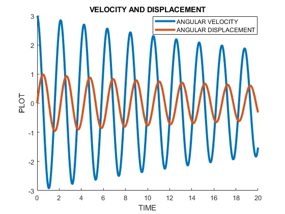
ploting time and result of ode column 1 (time and velocity ).ploting time and result of ode column 2.(time and displacement).
for creating of simulation first use for loop command
providing of x0 and y0 and x1 and y1 as starting cordinates and ending cordinates.
using of plot command to plot all component of the pendulum with their cordinetes .
for this note that any one of the plot should be written first then use hold comand to plot other plots.this will make the simulation smooth without repeatetive blurness see. example
plot([-1 1],[0 0],"b",LineWidth=10);
hold on
plot([0 0],[-1.3 0],"K:",LineWidth=2);
plot([x0 x1],[y0 y1],LineWidth=2,Color="k");
plot(x1,y1,"o",MarkerFaceColor="c",MarkerSize=20);
make sure of using hold off comand after plotting of all the plots.
to convert our plots in movie use m(ct)=getframe(gcf)
where ,
m is movie ,ct is frame of each plot , getframe comand ,gct is get current figure.
important ,ct=ct +1 should be after the m(ct)=getframe(gcf) comand so that first frame should be complet then series of in the loop.
movie(m) comand to generate movie.
to save the movie videofile=VideoWriter('name.avi',"Uncompressed AVI)
videofile=VideoWriter('name.avi',"Uncompressed AVI) instade of videofile=('name.avi',"Uncompressed AVI)
important ,ct=ct +1 should be after the m(ct)=getframe(gcf) comand so that first frame should be complet then series of in the loop.i had faced lot of error in this part after watching video i got it understand.
output plot
error recieved
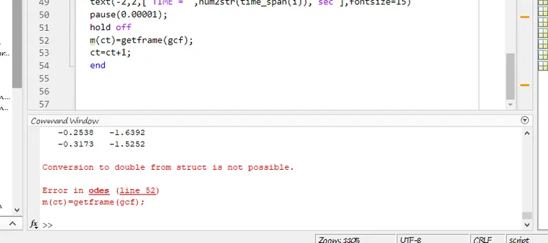
this was because i took (m) as a mass and (m) as a movie so need to change to (M).
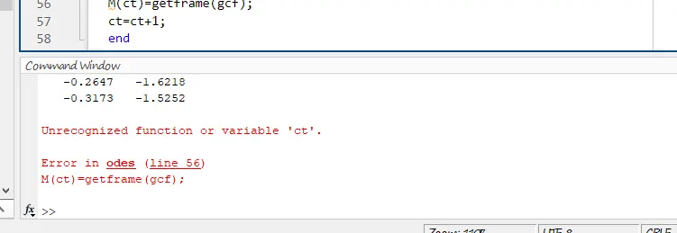
same error was come this was due to not adding ct=1 at starting of the for loop.
simulation of the video will be available on youtube
https://drive.google.com/file/d/1CaeRWd_0JX5kFduzgTJ-14TfDzLwCOfh/view?usp=sharing
THANK YOU