Project 1
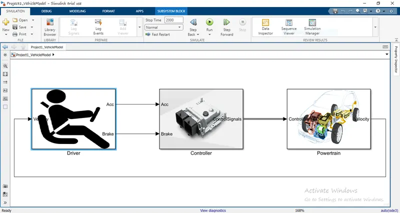
AIM: to compute the fuel economy numbers for the given vehicle (kmpl) on the urban cycle (UDDS) and highway cycle (HWFET). Also, to analyze and understand the vehicle operating.
what is conventional vehical ?
Gasoline and diesel vehicles are similar. They both use internal combustion engines. A gasoline car typically uses a spark-ignited internal combustion engine, rather than the compression-ignited systems used in diesel vehicles. In a spark-ignited system, the fuel is injected into the combustion chamber and combined with air. The air/fuel mixture is ignited by a spark from the spark plug. Although gasoline is the most common transportation fuel, there are alternative fuel options that use similar components and engine systems.

%%%%%%%%%%%%%%%%%%%%%%%%%%%%%%%%%%%%%%%%%%%%%%%%%%%%%%%%%%%%%%%%%%%%%
%% Skill-Lync -> Hybrid Drives Development
% Project 1 - Conventional Vehicle Model
% By - RITIK SONKAMBLE
clear all
close all
clc
% Description:

%% Initialization File
% Initialization file for loading the variables for the Conventional vehicle simulation model

%% Vehicle Parameters
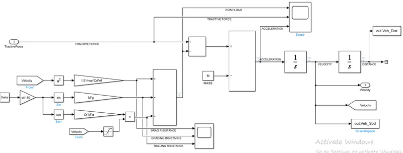
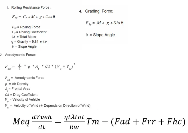
M = 1500;       % Vehicle weight [kg]
Cr = 0.015;     % Rolling resistance coefficient
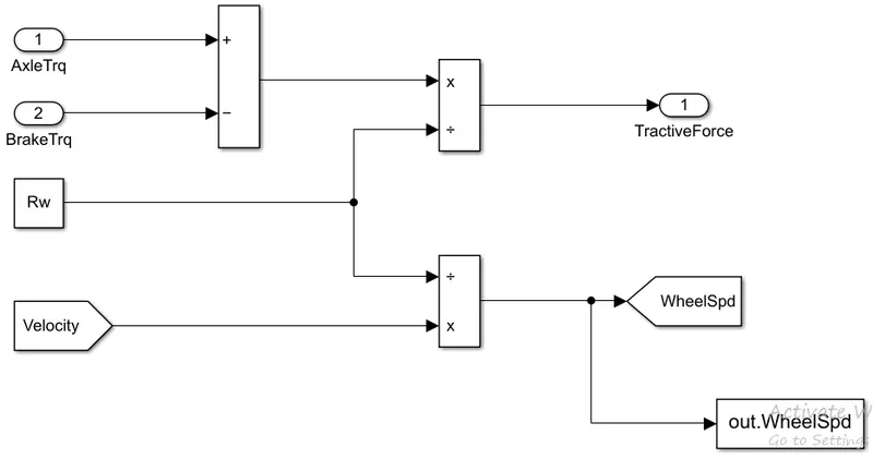
Rw = 0.35;      % Rolling radius [m]
Cd = 0.33;      % Drag coefficient
Af = 2;         % Frontal area [m2]
rhoa = 1.225;   % Air density [kg/m3]
Vwind = 0;      % Wind velocity [kmph]
g = 9.81;       % Gravitational acceleration [m/s2]
theta = 0;      % Slope [deg]
myu_road_tire = 1; % Coefficient of friction between tire - road interface

%% Powertrain Parameters
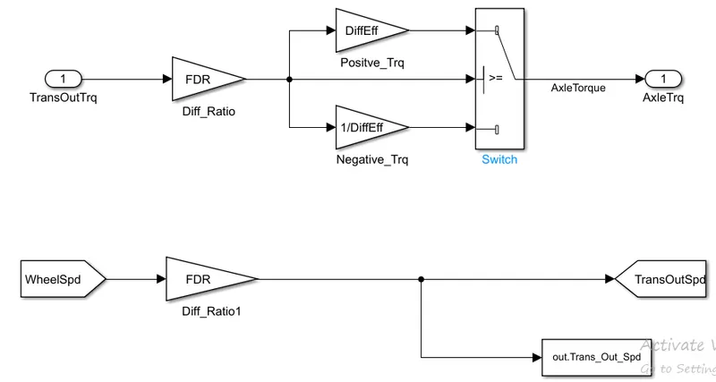
FDR = 3.73;                         % Final Drive Ratio / Diff Ratio
DiffEff = 0.99;                     % Differential efficiency (assumed independent of operating conditions)

NumGear = 4;                        % Number of gears in transmission
TransGear = [1:NumGear];            % Transmission Gears
TransRatio = [3.06, 1.62, 1, 0.7];  % Corresponding Transmission ratios
TransEff = 0.90;                    % Transmission efficiency (assumed independent of operating conditions)

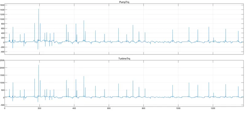
TC_SR = [0, .5, .6, .7, .8, .87, .92, .94, .96, .97, 1];   % Torque Converter Speed Ratio (Matlab default) -> TurbSpd/PumpSpd
TC_TR = [2.232, 1.5462, 1.4058, 1.2746, 1.1528, 1.0732, 1.0192, 1, 1, 1, 1];   % Torque Converter Torque Ratio (Matlab default) -> TurbTrq/PumpTrq
TC_Cf = 1e-4 * [.72558, .66322, .63463, .59042, .51331, .4144, .29287, .22444, .12186, .04386, 0]; % Torque Converter Capacity Factor (Matlab default) -> PumpTrq/PumpSpd^2 [Nm/rpm^2]

load Vehicle_Data/Engine_data_1_9L_Saturn_95kW
load Vehicle_Data/Trans_Shift_map

%% Driver Parameters
Kp = 10;                    % P gain for driver PI model
Ki = 1;                     % I gain for driver PI model
Drive_Cycle_Select = 1   % Drive cycle selection

% Drive cycle values in m/s

if Drive_Cycle_Select == 1
    load DriveCycles/UDDS;
    fprintf('UDDS CYCLE IS LOADED \n')

elseif Drive_Cycle_Select == 2
    load DriveCycles/HWFET;
     fprintf('HWFET CYCLE IS LOADED \n')

elseif Drive_Cycle_Select == 3
    load DriveCycles/FTP;
     fprintf('FTP CYCLE IS LOADED \n')

elseif Drive_Cycle_Select == 4
    load DriveCycles/US06;
     fprintf('US06 CYCLE IS LOADED \n')

elseif Drive_Cycle_Select == 5
    load DriveCycles/NEDC;
     fprintf('NEDC CYCLE IS LOADED \n')

elseif Drive_Cycle_Select == 6
    load DriveCycles/WLTP;
     fprintf('WLTP CYCLE IS LOADED \n')

end

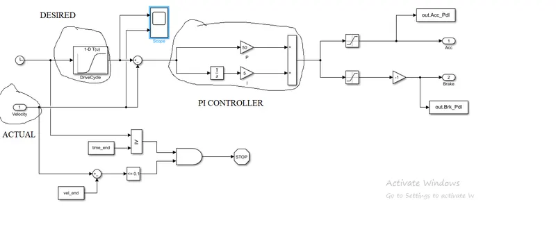
time_end = cyc_time(end);
vel_end = cyc_vel(end);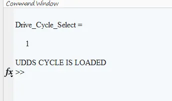
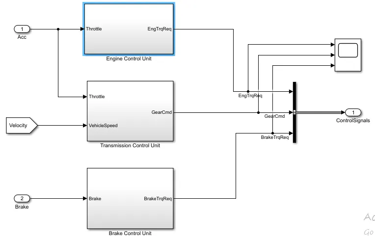
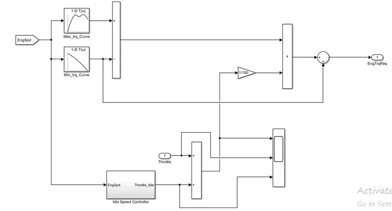
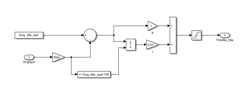
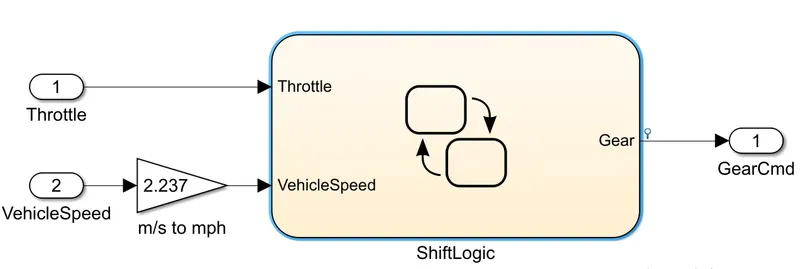
%%%%%%%%%%%%%%%%%%%%%%%%%%%%%%%%%%%%%%%%%%%%%%%%%%%%%%%%%%%%%%%%%%%%%
%% Skill-Lync -> Hybrid Drives Development
% Project 1 - Conventional Vehicle Model
% By - RITIK SONKAMBLE


%% Post-Processing File
%  File for post-processing the Conventional vehicle simulation model data

%% Renaming variables
Time = out.tout;
Acc_Pdl = out.Acc_Pdl;          % Accelerator pedal [%]
Brk_Pdl = out.Brk_Pdl;          % Brake pedal [%]
Gear_Cmd = out.Gear_Cmd;        % Transmission gear
Trans_In_Spd = out.Trans_In_Spd*30/pi;  % Transmission input speed [rpm]
Trans_Out_Spd = out.Trans_Out_Spd*30/pi;% Transmission output speed [rpm]
Eng_Trq = out.Eng_Trq;          % Engine brake torque [Nm]
Eng_Spd = out.Eng_Spd*30/pi;    % Engine speed [rpm]
Eng_Fuel_Consump = out.Eng_Fuel_Consumption;    % Engine fuel consumption [g]
Veh_Dist = out.Veh_Dist/1000;   % Distance traveled by vehicle [km]
Veh_Spd = out.Veh_Spd*18/5;     % Vehicle speed [kmph]
WheelSpd=out.WheelSpd;            % wheel speed [rpm]
Eng_Fuel_rate=out.Eng_Fuel_Rate;
%% Data Analysis
Eng_Pwr = Eng_Spd.*pi./30.*Eng_Trq./1000;   % Engine brake power [kW]
rho_petrol = 0.7197;                    % Density of petrol [kg/L]
kmpl = Veh_Dist(end)/(Eng_Fuel_Consump(end)/1000/rho_petrol);    % Fuel economy [kmpl]

%% TIME TRACT FOR ENGINE
figure(1)
hold on
grid on
plot(Time,Trans_In_Spd, 'linewidth', 1, 'Color', 'black')
plot(Time,Trans_Out_Spd, 'linewidth', 1, 'Color', 'red')
plot(Time,WheelSpd, 'linewidth', 1, 'Color', 'green')
xlabel('time [s]')
ylabel('speed [rpm]')
xlim([0, Time(end)]);
ylim([0, 6000]);
legend('Trans In Spd','Trans Out Spd','WheelSpd')
%% Plotting torque ,power,fuel rate,fuel consumption
figure(2)
subplot(4,1,1)
grid on
plot(Time, Eng_Trq, 'linewidth', 1, 'Color', 'black');
xlabel('time [s]')
ylabel('engine torque [Nm]')
xlim([0, Time(end)]);
subplot(4,1,2)
grid on
plot(Time, Eng_Pwr, 'linewidth', 1, 'Color', 'blue');
xlabel('time [s]')
ylabel('engine power [Nm]')
xlim([0, Time(end)]);
subplot(4,1,3)
grid on
plot(Time,Eng_Fuel_rate, 'linewidth', 1, 'Color', 'green');
xlim([0, Time(end)]);
xlabel('Time [s]');
ylabel('engine fuel rate');
subplot(4,1,4)
grid on
plot(Time,Eng_Fuel_Consump, 'linewidth', 1, 'Color', 'red');
xlim([0, Time(end)]);
xlabel('Time [s]');
ylabel('engine fuel consumption');
%% Plotting vehicle characteristics time trace
figure(3)
subplot(4,1,1)
hold on
grid on
plot(Time, Acc_Pdl, 'linewidth', 1, 'Color', 'black');
plot(Time, Brk_Pdl, 'linewidth', 1, 'Color', 'red');
ylabel('Pedal [%]')
xlim([0, Time(end)]);
legend('Accel','Brake');
subplot(4,1,2)
hold on
grid on
plot(Time, Gear_Cmd, 'linewidth', 1, 'Color', 'black');
xlim([0, Time(end)]);
xlabel('Time [s]');
ylabel('Gear');
subplot(4,1,3)
hold on
grid on
plot(cyc_time,(cyc_vel.*(18./5)), 'linewidth', 1, 'Color', 'black');
plot(Time, Veh_Spd, 'linewidth', 1, 'Color', 'red');
ylabel('velocity')
xlabel('Time [s]');
xlim([0, Time(end)]);
legend('desired speed','Actual speed');
subplot(4,1,4)
hold on
grid on
plot(Time, Veh_Dist, 'linewidth', 1, 'Color', 'black');
xlim([0, Time(end)]);
xlabel('Time [s]');
ylabel('distance [km]');

%% Plotting engine operating points on engine fuel map
figure('Name','Engine Operating Points');
hold on
grid on
title('Engine Operating Points','fontsize',12);
p1=plot(Eng_map_spd*30/pi,Eng_max_trq,'linewidth',2,'color','r');
p2=line([Eng_map_spd(end)*30/pi Eng_map_spd(end)*30/pi],[0 Eng_max_trq(end)]);
set(p2,'linewidth',1,'linestyle','--','color','k');
p3=line([Eng_map_spd(1)*30/pi Eng_map_spd(1)*30/pi],[0 Eng_max_trq(1)]);
set(p3,'linewidth',1,'linestyle','--','color','k');
[c,h] = contour(Eng_map_spd'*30/pi,Eng_map_trq,Eng_fuel_map');
clabel(c,h);
xlabel('Engine Speed [rpm]');
ylabel('Engine Torque [Nm]');
title('Engine Fuel Consumption Map [g/s]');
p4 = plot(Eng_Spd,Eng_Trq,'.','color','k');
legend([p1 p4],{'Max Curve','Operating Points'});
axis([Eng_map_spd(1)*30/pi Eng_map_spd(end)*30/pi 0 Eng_map_trq(end)]);
in this code we will plotthe values that are extracted from the simulink model and compair it with {UDDS CYCLE VS HWFET CYCLE}
WE WILL SEE PLOT FOR
1. Tabulate the fuel economy numbers (kmpl) for UDDS and HWFET cycle.
2. Plot the time trace for engine, transmission input, transmission output and wheel speed on one plot.
3. Plot engine torque, engine power, fuel rate and fuel consumption using subplots.
4. Plot accelerator and brake pedal, gear command, vehicle desired and actual speed,vehicle distance using subplots.
5. Plot the engine operating points on the engine fuel map.
1. Tabulate the fuel economy numbers (kmpl) for UDDS and HWFET cycle.
fuel economy numbers (kmpl) for UDDS cycle = 16.8534
fuel economy numbers (kmpl) for HWFET cycle = 21.2041
fuel economic number is in HWFET cycly is higher because ther is low pealing which cause low energy loss which cause less fuel consumption where as as compaire to UDDS cycle there is more pedeling means more energy loss due to loss which cause more fuel consumption .
2. Plot the time trace for engine, transmission input, transmission output and wheel speed on one plot.
in the below figure1 we there is more fluctuation in speed .means transmisson speed is decreasing to zero in every few time which cause less out energy generation .as compaire to figure 2 we can see that there is less fluctuation means transmission speed is very low to zero for long period of time which produce more energy. we can see this in figure no 5 AND 6 FIRST PLOT.
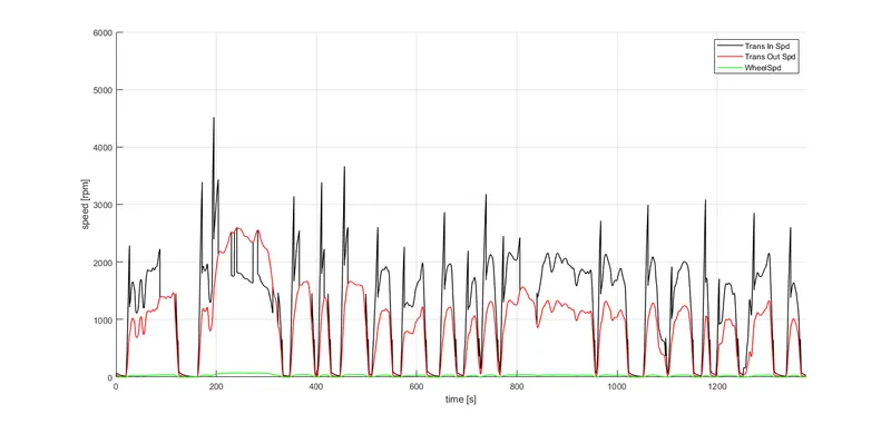
FIGURE 1 : engine, transmission input, transmission output and wheel speed FOR UDDS CYCLE
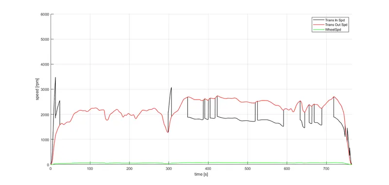
FIGURE 2 : engine, transmission input, transmission output and wheel speed FOR HWFET CYCLE.
3 . Plot engine torque, engine power, fuel rate and fuel consumption using subplots.
in figure 3 and 4 we can see the engine torque, engine power, fuel rate is directly proportional to each other . which means as engine power is increased the torque is also increased and at time fuel rate is also increase the main difference between figure 3 and 4 is fluctuation due to instant increase and decrease in power,torque ,fuel rate. due to the driving condition.
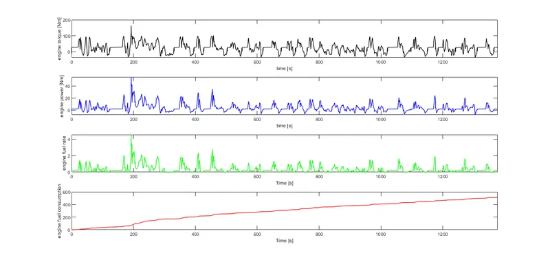
FIGURE 3: engine torque, engine power, fuel rate and fuel consumption FOR UDDS CYCLE
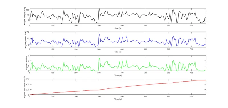
FIGURE 4: engine torque, engine power, fuel rate and fuel consumption FOR HWFET CYCLE
4. Plot accelerator and brake pedal, gear command, vehicle desired and actual speed,vehicle distance using subplots.
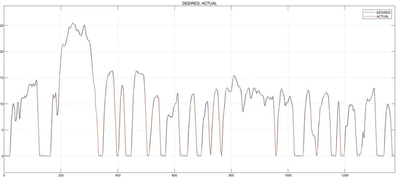
in figure 5 we can see that if the gear is not constant for long period we will recieve less velocity where as in figure 6 the gear is constant for long period means velocity is also increasing due to which there is less pedeling and cause less power loss. by looking at the graph 5 and 6 we can identify that vehical is stopped multipal time in a given distance due to zero velocity at multipal time for UDDS cycle where as in HWFET cycle no vehical stop multipal time in given diastance due to gradually increasing and decreasing in velocity without making it zero.
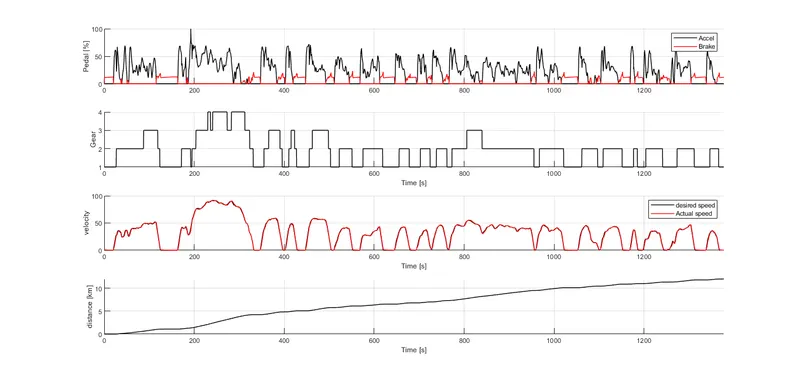
FIGURE 5: accelerator and brake pedal, gear command, vehicle desired and actual speed,vehicle distance for UDDS CYCLE
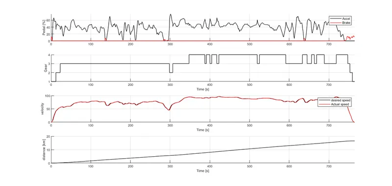
FIGURE 6: accelerator and brake pedal, gear command, vehicle desired and actual speed,vehicle distance for HWFET CYCLE.
5. Plot the engine operating points on the engine fuel map.
from the below figures we can see that in UDDS CYCLE engine operating point are exceding the max curve wher as in HWFET CYCLE the engine operating points are low. in both the figure we can see that there is much nigher RPM is availabe which is not used 60000.
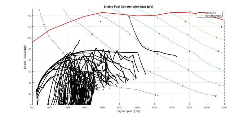
FIGURE 7: Engine operating points FOR UDDS CYCLE
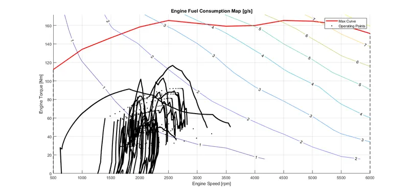
FIGURE 8: Engine operating points FOR HWFET CYCLE
link to access :
https://drive.google.com/drive/folders/1ZArTjjUGOk4YBlhz09DL-IuPuLY7SyXn?usp=sharing
CONCLUSION:
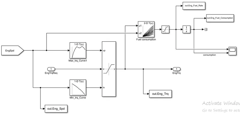
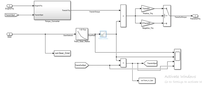
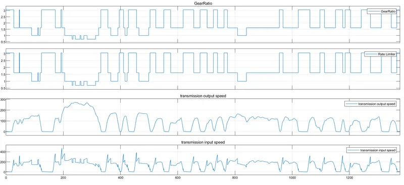
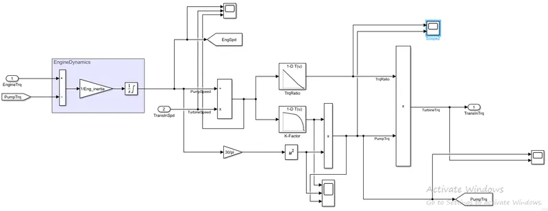
hence i we have tudied how Conventional Vehicle Model is designed and work by using matlab coding and and matlab simulink.
we had studyed how the graph of the vehical is plotted with different drive cycle .
THANK YOU