Project 2 - Rankine cycle Simulator
Project 2 - Rankine cycle Simulator
AIM:- Rankine cycle Simulator
OBJECTIVE :-
- Create a Rankine Cycle Simulator.
- state points of the Rankine Cycle (any type of your choice) based on user inputs.
- Then, plot the corresponding T-s and h-s plots for the given set of inputs.
- report explaining the working of a rankine cycle simulation.
WHAT IS RANKINES CYCLE?
The Rankine Cycle is a mechanical cycle commonly used in power plants to convert the pressure energy of steam into mechanical energy through steam turbine. The Rankine Cycle’s major components include a rotating steam turbine, a boiler pump, a stationary condenser, and a boiler.
A boiler is used to heat the water for steam at the required pressure and temperature as per the turbine’s requirement for power generator.
The turbine exhaust is directed to the radial or axial flow condenser for condensing the steam to condensate and recycled back to the boiler through boiler pumps for heating again.
T/S diagram
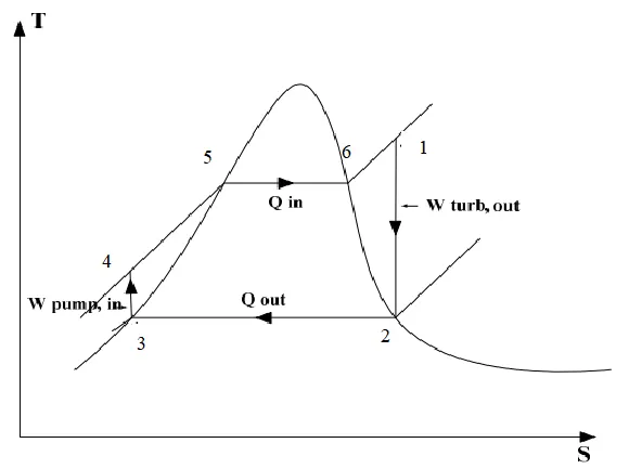
in the above digram
1 -2 is the work done by turbine in which high temperature high pressure vapour gives the output work and due to which its temperature and pressure is decreased.
2-3 is the process in which vapour is passed into condenser to convert vapour to liquid with constant pressure.
3-4 is the process in which temprature and pressure is increased in very less amount due to work done on water to pump it on the boiler.
4-5 is the process in which liquid temperature is increased in the boiler and at one point it stop increassing temperature for phase change.(work done in the boiler)
5-6 is the phase change process from liquid to vapour with constant temperature changing phase.(work done in the boiler)
6-1 when the liquid is converted into vapour temperature is increased then it is send in the turbine to give work.(work done in the boiler).
formulas for calculations
turbine_work=h1-h2
pump_work=h4-h3
heat_input=h1-h4
heat_output=h2-h1
net_work=turbine_work-pump_work
effiency=(net_work/heat_input)*100
back_work_ratio=pump_work/turbine_work
PROGRAM:-
clear all
close all
clc


disp('                       RANKINE CYCLE SIMULATOR      ')

fprintf('\n1-2 IS ISENTROPIC EXPANSION IN THE TURBINE\n')
disp('2-3 IS CONSTANT PRESSURE HEAT REJECTION BY THE CONDENSER')
disp('3-4 IS ISENTROPIC COMPRESSION IN THE PUMP')
disp('4-1 IS CONSTANT PRESSURE HEAT ADDITION BY THE BOILER')

% %Required Inputs:
t1=400;
p1=30;
p2=0.05;

fprintf('\n\nINPUTS')
fprintf('\nENTER THE PRESSURE AT THE TURBINE INLET (IN BAR) %.2f:',p1)
fprintf('\nENTER THE TEMPERATURE AT THE TURBINE INLET (IN DEGREE CELCIUS): %.2f',t1)
fprintf('\nENTER THE PRESSURE AT THE CONDENSER (IN BAR): %.2f',p2)


 % stage 1

h1=XSteam('h_pT',p1,t1);  % enthalpy at 1
s1=XSteam('s_pT',p1,t1);  % entropy at 1
tsat=XSteam('tsat_p',p1); % saturation temperature

 % stage 2
s2=s1;                     % isentropic process 1-2
t2=XSteam('T_ps',p2,s2);   % temperature at 2
sf2=XSteam('sL_p',p2);     % saturated liquid entropy
sg2=XSteam('sV_p',p2);     % saturated vapor entropy
x=(s2-sf2)/(sg2-sf2);      % dryness factor
hf2=XSteam('hL_p',p2);     % saturated liquid enthalpy
hg2=XSteam('hV_p',p2);     % saturated vapour enthalpy
h2=hf2+ x*(hg2-hf2);       % enthalpy at 2

% stage 3
t3=t2;  % temperature at 3
p3=p2;  % pressure at 3
s3=sf2; % entropy at 3
h3=hf2; % enthalpy at 3

% stage 4
p4=p1;                        % isobaric process 4-1
s4=s3;                        % isentropic process 3-4
h4=XSteam('h_ps',p4,s4);      % enthalpy at 4
t4=XSteam('t_ps',p4,s4);      % temperature at 4

%stage 5 and 6 for the curve
s5=XSteam('sL_p',p4);       % Saturated liquid entropy at 5
h5=XSteam('hL_p',p4);       % Saturated liquid enthalpy at 5
t5=XSteam('Tsat_p',p4);     % Saturation temperature at 6
s6=XSteam('sV_p',p4);       % Saturated vapour entropy at 6
h6=XSteam('hV_p',p4);       % Saturated vapour enthalpy at 6
t6=t5;                      % temperature at 6

%% preparing curve for T and S , and S and H
t=linspace(1,400,1000);
for i=1:length(t)
    sf(i)=XSteam('sL_T',t(i));  %Saturated liquid entropy
    sg(i)=XSteam('sV_T',t(i));  %Saturated vapour entropy
    hf(i)=XSteam('hL_T',t(i));  %Saturated liquid enthalpy
    hg(i)=XSteam('hV_T',t(i));  %Saturated vapour enthalpy
end

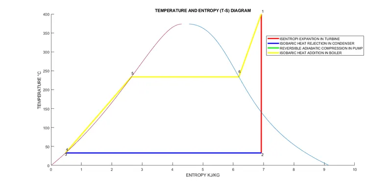
%% PLOTTING  OF ENTROPY AND TEMPERATURE
figure(1)
hold on
plot([s1,s2],[t1,t2],Color='r',LineWidth=3)
plot([s2,s3],[t2,t3],Color='b',LineWidth=3)
plot([s3,s4],[t3,t4],Color='g',LineWidth=3)
plot([s4,s5],[t4,t5],Color='y',LineWidth=3)
plot([s5,s6],[t5,t6],Color='y',LineWidth=3)
plot([s6,s1],[t6,t1],Color='y',LineWidth=3)
plot(sf,t)
plot(sg,t)
xlabel('ENTROPY KJ/KG')
ylabel('TEMPERATURE °C ')
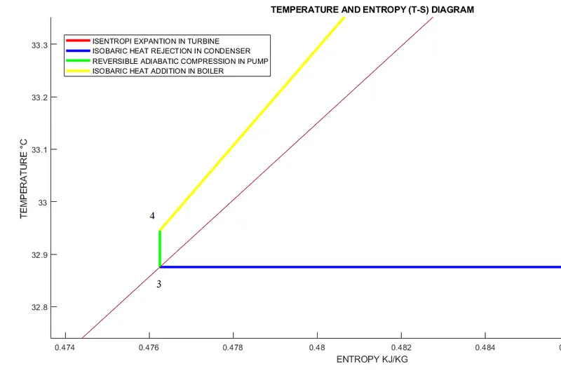
legend('ISENTROPI EXPANTION IN TURBINE','ISOBARIC HEAT REJECTION IN CONDENSER','REVERSIBLE ADIABATIC COMPRESSION IN PUMP','ISOBARIC HEAT ADDITION IN BOILER')
title('TEMPERATURE AND ENTROPY (T-S) DIAGRAM')
hold off
gtext('1')
gtext('2')
gtext('3')
gtext('4')
gtext('5')
gtext('6')
%% PLOTTING OF ENTROPY AND ENTHALPY GRAPH
figure(2)
hold on
plot(sg,hg,LineWidth=3)
plot(sf,hf,LineWidth=3)
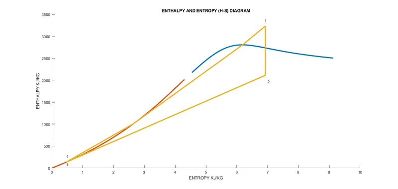
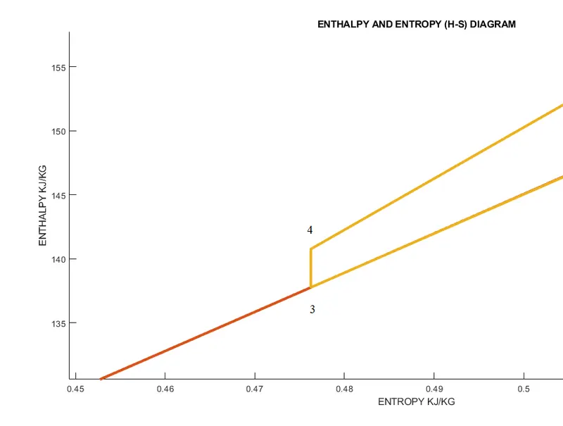
plot([s1,s2,s3,s4,s5,s6,s1],[h1,h2,h3,h4,h5,h6,h1],LineWidth=3)
xlabel('ENTROPY KJ/KG')
ylabel('ENTHALPY KJ/KG')
title('ENTHALPY AND ENTROPY (H-S) DIAGRAM')
hold off
gtext('1')
gtext('2')
gtext('3')
gtext('4')

%% CALCULATIONS
turbine_work=h1-h2;
pump_work=h4-h3;
heat_input=h1-h4;
heat_output=h2-h1;
net_work=turbine_work-pump_work;
effiency=(net_work/heat_input)*100;
ssc=(3600/net_work);
back_work_ratio=pump_work/turbine_work;


disp(' ')
disp('-----------------------------------------------------------------------------------------------------')
disp('                                                        RESULT               ')
fprintf('\nAT STATE POINT 1 :\n' )
fprintf('P1 IS : %.2f bar \n',p1)
fprintf('T1 IS : %.2f °C\n',t1)
fprintf('H1 IS : %.2f kj/kg\n',h1)
fprintf('S1 IS : %.2f Kj/kgk\n',s1)

fprintf('\nAT STATE POINT 2 :\n' )
fprintf('P2 IS : %.2f bar \n',p2)
fprintf('T2 IS : %.2f °C\n',t2)
fprintf('H2 IS : %.2f kj/kg\n',h2)
fprintf('S2 IS : %.2f Kj/kgk\n',s2)

fprintf('\nAT STATE POINT 3 :\n' )
fprintf('P3 IS : %.2f bar\n',p3)
fprintf('T3 IS : %.2f °C\n',t3)
fprintf('H3 IS : %.2f kj/kg\n',h3)
fprintf('S3 IS : %.2f Kj/kgk\n',s3)

fprintf('\nAT STATE POINT 4 :\n' )
fprintf('P4 IS : %.2f bar\n',p4)
fprintf('T4 IS : %.2f °C\n',t4)
fprintf('H4 IS : %.2f kj/kg\n',h4)
fprintf('S4 IS : %.2f Kj/kgk\n',s4)

fprintf('\nTURBINE WORK IS               :  %.4f kj/kg\n',turbine_work)
fprintf('PUMP WORK IS                  :  %.4f kj/kg\n',pump_work)
fprintf('NET WORK IS                   :  %.4f kj/kg\n',net_work)
fprintf('THERMAL EFFENCY IS            :  %.4f ٪ \n',effiency)
fprintf('SPECIFIC STEAM CONSUMPTION IS :  %.4f kg/kwh\n',ssc)
fprintf('BACK WORK RATIO IS            :  %.4f \n',back_work_ratio)
EXPLANATION OF PROGRAM:-
using of disp and fprintf command to display the written concept int he window.
using disp command to provide proper spacing in in command window.
providing of input values which are t1,p1,p2.
using the fprintf command after the input so that every time we change input we can get the result shown in the command window.
stage 1 ,stage 2 ,stage 3 ,stage 4 ,stage 5,6
extracting the values of the temperature ,enthalpy ,entropy from xsteam file at each stage with proper input of the required stage input as pressure , temperature .
(example t2=XSteam('T_ps',p2,s2)
where t2 is the temperature we need =xstream is the function name ,t_ps is the temperature as a function of pressure and entropy.)
creating temperature range for the curve .
providing a for loop for getting values of liquid and vapour for enthalpy an entropy so with respective to temperature.
using figure comand tho get seprate figure.
hold on command to plot all the points on same figure.
first way of ploting comand
plot([s1,s2],[t1,t2]) where [] this bracket to provide all the x values first then the y values second.
plot (sf,t) which gives the curves in the figure.
providing xlable, ylable, legends, title
then hold off comand.
gtext comand to add text when taped on the graph.
second way of potting graph is providing all the values in one plot comand.
example this
plot([s1,s2,s3,s4,s5,s6,s1],[h1,h2,h3,h4,h5,h6,h1],LineWidth=3)
dis advantage of this is cannot able to give seprate inne colour due do which cannot provide legends.
using formulas for the calculation.
using of display comand to display the text .
then using fprintf comand to pring the values .
example:
fprintf('P1 IS : %.2f bar \n',p1)
P1 IS : is the text to be printed ,%.f is to print the floting no ,(.2) is to print 2 number after point, \n is to go in next line, p1 is the input value to be printed.
Calculate the followings
Net work output=1117.8657 kj/kg
Back work ratio=0.0027
COMMAND WINDOW :-
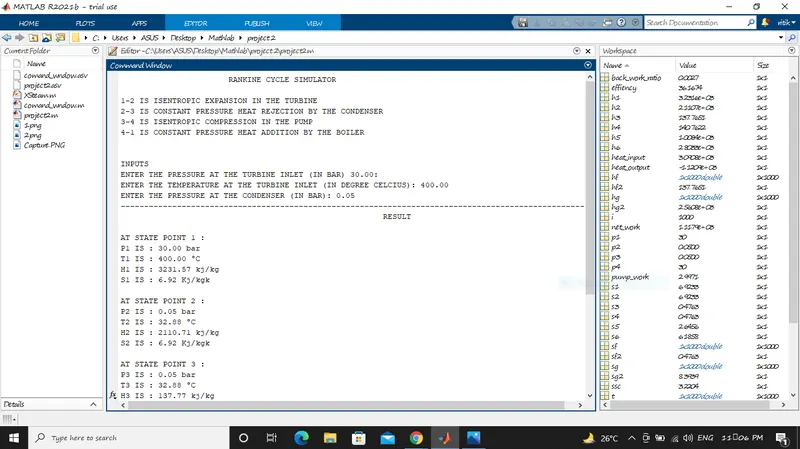
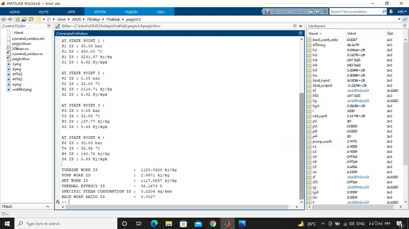
TEMPERATURE v/s ENTROPY T-S DIAGRAM
ENTHALPY v/s ENTROPY H-S DIAGRAM :-
errors:
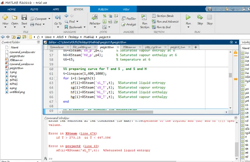
this was the longest error faced by me i ind put t(i)
CONCLUSION:
successfully Create a Rankine Cycle Simulator using MATLAB. with T/S and H/S diagram.
REFERENCES:-
https://www.electrical4u.com/ideal-verses-actual-in-rankine-cycle/
https://mechanicalboost.com/rankine-cycle/
thank you