Project 2

AIM:- the development of a forward energy-based fuel consumption model of a P1 hybrid vehicle and understand the functionality of a P1 hybrid and be able to model it by using matlab and simulink.

OBJECTIVE

1. Write a project report that contains the following:
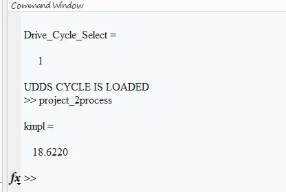
2. Tabulate the fuel economy numbers (kmpl) for UDDS and HWFET cycle. Compare these numbers with the baseline numbers for conventional vehicle model from Project 1.
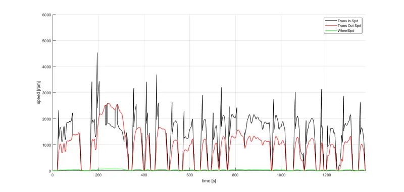
3. Plot the time trace for engine, transmission input, transmission output and wheel speed on one plot.
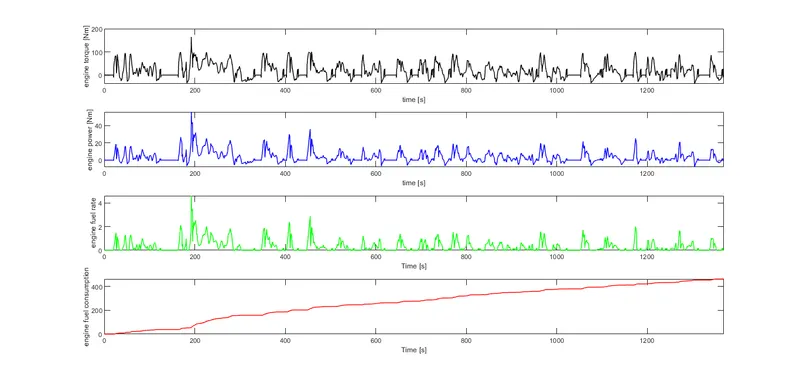
4. Plot engine torque, engine power, fuel rate and fuel consumption using subplots.
5. Plot accelerator and brake pedal, gear command, vehicle desired and actual speed, vehicle distance using subplots.
6. Plot the engine operating points on the engine fuel map.
7. Plot motor speed, torque, motor input power using subplots.
8. Plot pack voltage, current and SoC using subplots.
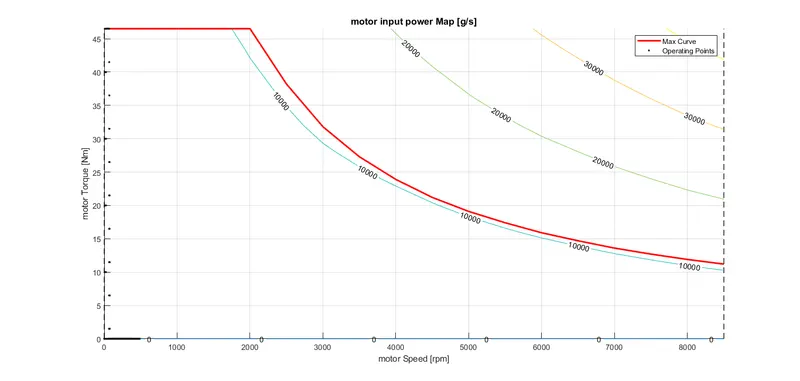
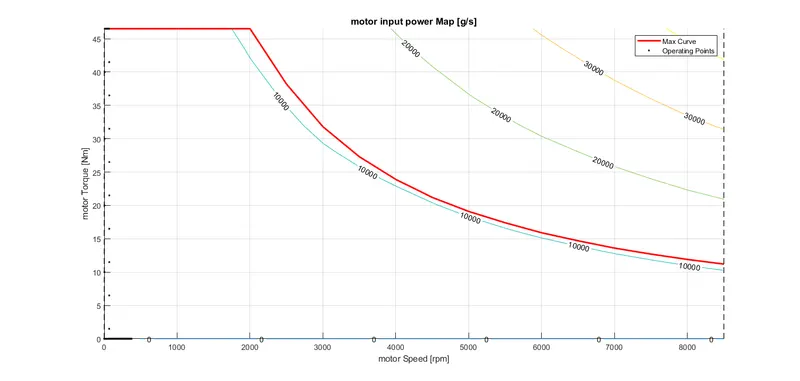
9. Plot the motor operating points on the motor input power map, with the motor max motoring and generating torque curves.

WHAT IS P1 HYBRID ELECTRIC VEHICAL ?

The P1 architecture, with the electric machine connected directly to the crankshaft, is the solution adopted by Honda on their first generation Integrated Motor Assist (IMA) technology. The electric motor functions as a generator, during vehicle deceleration, as an engine starter, and as a motor (to assist the engine) during vehicle accelerations.

One of the biggest advantage of this solution is that the electric motor can provide higher torque than the BiSG, since there is no belt limitation (due to slip). However, since there is no speed / torque ratio between the electric machine and crankshaft, the torque requirements on the electric motor can be quite demanding.

Two examples of P1 MHEV architectures are:

• Honda Insight Hybrid 2009 (with Integrated Motor Assist technology)
• Mercedes Benz S400 Bluehybrid 2010

TYPES.

P0	The electric machine is connected with the internal combustion engine through a belt, on the front end accessory drive (FEAD)
P1	The electric machine is connected directly with the crankshaft of the internal combustion engine
P2	The electric machine is side-attached (through a belt) or integrated between the internal combustion engine and the transmission; the electric machine is decoupled from the ICE and it has the same speed of the ICE (or multiple of it)
P3	The electric machine is connected through a gear mesh with the transmission; the electric machine is decoupled from the ICE and it’s speed is a multiple of the wheel speed
P4	The electric machine is connected through a gear mesh on the rear axle of the vehicle; the electric machine is decoupled form the ICE and it’s located in the rear axle drive or in the wheels hub

MY CODES:

%% Skill-Lync -> Hybrid Drives Development
clear all
 close all
 clc

%% Skill-Lync -> Hybrid Drives Development
% Project 2 - P1 hybrid Vehicle Model
% By - RITIK SONKAMBLE

%% Vehicle Parameters
M = 1500;       % Vehicle weight [kg]
Cr = 0.015;     % Rolling resistance coefficient
Rw = 0.35;      % Rolling radius [m]
Cd = 0.33;      % Drag coefficient
Af = 2;         % Frontal area [m2]
rhoa = 1.225;   % Air density [kg/m3]
Vwind = 0;      % Wind velocity [kmph]
g = 9.81;       % Gravitational acceleration [m/s2]
theta = 0;      % Slope [deg]
myu_road_tire = 1; % Coefficient of friction between tire - road interface

%% Powertrain Parameters 
FDR = 3.73;                         % Final Drive Ratio / Diff Ratio
DiffEff = 0.99;                     % Differential efficiency (assumed independent of operating conditions)

NumGear = 4;                        % Number of gears in transmission
TransGear = [1:NumGear];            % Transmission Gears
TransRatio = [3.06, 1.62, 1, 0.7];  % Corresponding Transmission ratios
TransEff = 0.90;                    % Transmission efficiency (assumed independent of operating conditions)

TC_SR = [0, .5, .6, .7, .8, .87, .92, .94, .96, .97, 1];   % Torque Converter Speed Ratio (Matlab default) -> TurbSpd/PumpSpd  
TC_TR = [2.232, 1.5462, 1.4058, 1.2746, 1.1528, 1.0732, 1.0192, 1, 1, 1, 1];   % Torque Converter Torque Ratio (Matlab default) -> TurbTrq/PumpTrq
TC_Cf = 1e-4 * [.72558, .66322, .63463, .59042, .51331, .4144, .29287, .22444, .12186, .04386, 0]; % Torque Converter Capacity Factor (Matlab default) -> PumpTrq/PumpSpd^2 [Nm/rpm^2]

load Vehicle_Data/Engine_data_1_9L_Saturn_95kW
load Vehicle_Data/Trans_Shift_map
load Vehicle_Data/EM_Honda_Insight_10kW
load Vehicle_Data/ESS_NiMH6

ESS_init_soc = 0.8;
ESS_soc_max = 0.9;
ESS_soc_min = 0.6;



%% Driver Parameters
Kp = 10;                    % P gain for driver PI model
Ki = 1;                     % I gain for driver PI model
Drive_Cycle_Select = 1     % Drive cycle selection

% Drive cycle values in m/s

if Drive_Cycle_Select == 1
    load DriveCycles/UDDS;
    fprintf('UDDS CYCLE IS LOADED \n')

elseif Drive_Cycle_Select == 2
    load DriveCycles/HWFET;
    fprintf('HWFET CYCLE IS LOADED \n')

elseif Drive_Cycle_Select == 3
    load DriveCycles/FTP;
    fprintf('FTP CYCLE IS LOADED \n')

elseif Drive_Cycle_Select == 4
    load DriveCycles/US06;
    fprintf('US06 CYCLE IS LOADED \n')
    
elseif Drive_Cycle_Select == 5
    load DriveCycles/NEDC;
    fprintf('NEDC CYCLE IS LOADED \n')

elseif Drive_Cycle_Select == 6
    load DriveCycles/WLTP;
    fprintf('WLTP CYCLE IS LOADED \n')
 
end

time_end = cyc_time(end);
vel_end = cyc_vel(end);

the above code are the initial file which contain all the input values which are required to develop a simulink model.

the codes are loading the files which contain data of Engine_data,Trans_Shift,EM_Honda_Insight_10kW,ESS.

the data of different dive cycle are also loaded and condition is given that if we put 1,... the perticular drive cycle data will be get loaded.

once we run this file all the data will be stored and now we can go to simulink model.

simulink model

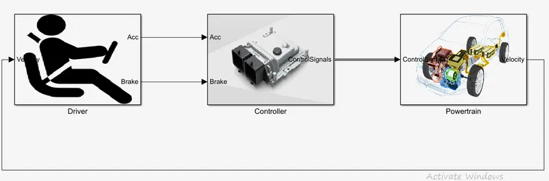
the above figure show the driver control block which generates the accelration, brake.

controller block which is electronic control unit which takes the driver input and figures out the Engine, transmission, electric motor ,break need to be provided .

power train block consist of engine ,transmission,differential,wheel and vehical dynamic,motor, ess,crankshaft which are calculated on the basis of torque requirement ,gear ratio,break torque .

inside of controller

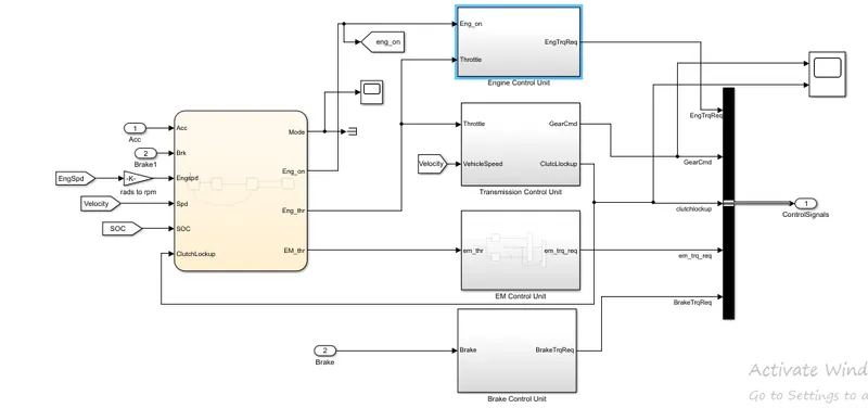
inside view of the controller block lets explore these all blocks.

FLOW CHART

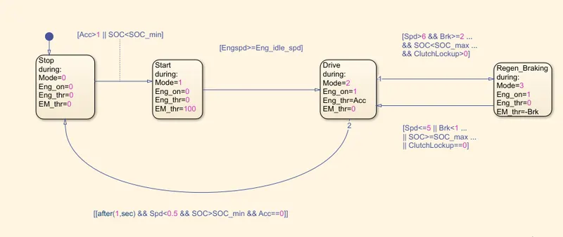
in this flow chat we are providing the modes 0,1,2,3 each stages and to go from one stage to another there is some condition is given.

where inside the block are the output need when the condition will be satisfing and the condition are the input.

example

the vehcial will be in stop stage where the engine on , engine throttle ,electric moter will be 0.

when the Acceleration is grater than 1 or SOC < SOC_min it will go to next stage.

and so on...

ENGINE CONTROL UNIT:

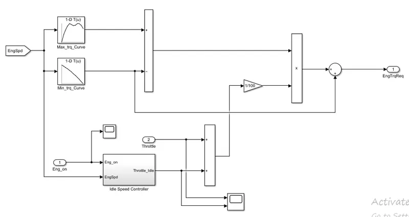
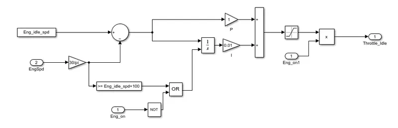
in engine block the idle speed controller block is edited and add eng on so that we can dissable the ideal speed controller when the engine is off it get zero .so that we should not get any torque request.

TRANSMISSION CONTROL UNIT

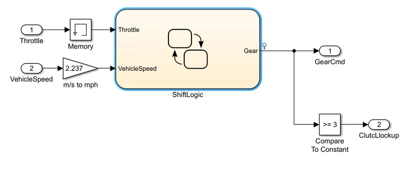
memory block is added over hear to provide delay as an input.output of the gear command is taken as clutch lock up with compair to constant block where the 3 is the gear no. the moto of using this block is in automatic transmission we need to lock clutch as soon as possible but it is not easy to do because at low speed the pump do not have enough pressure to lock it up. 1000-2000 rpm and another reason lots of torque multi is happning which causes lots of vibration.

ELECTRIC MOTOR CONTROLLER

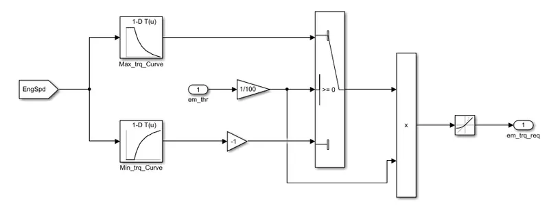
this block desides how much torque need to be get.

POWER TRAIN

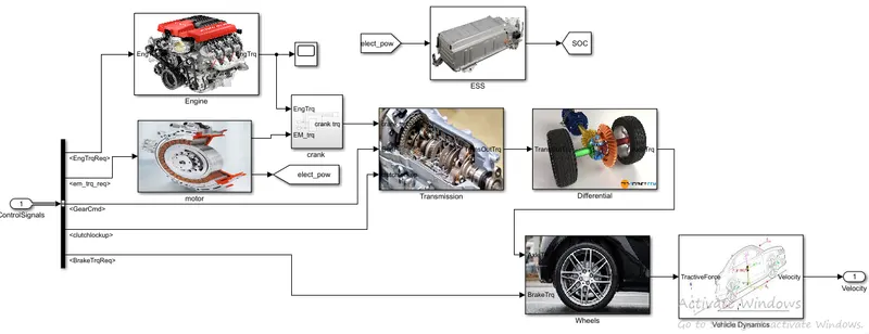
ENGINE

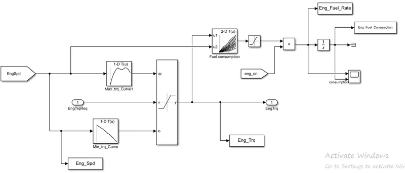
engine on value is added here so that when the engine is off the it will multiply with zero and give zero fuel consumption.and also not to get extrapolation errors.

MOTOR

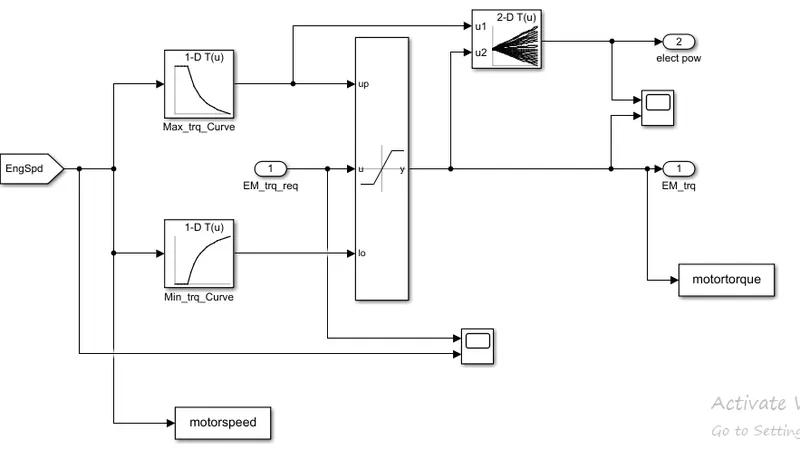
calculation of motor toque and motor power is don here.

CRANK HUB

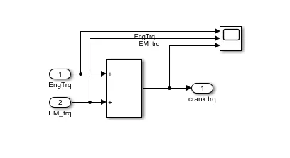
here we are adding both the torque gettng from engine and from motor and sending to transmission.

ESTIMATED STORAGE SYSTYEM.

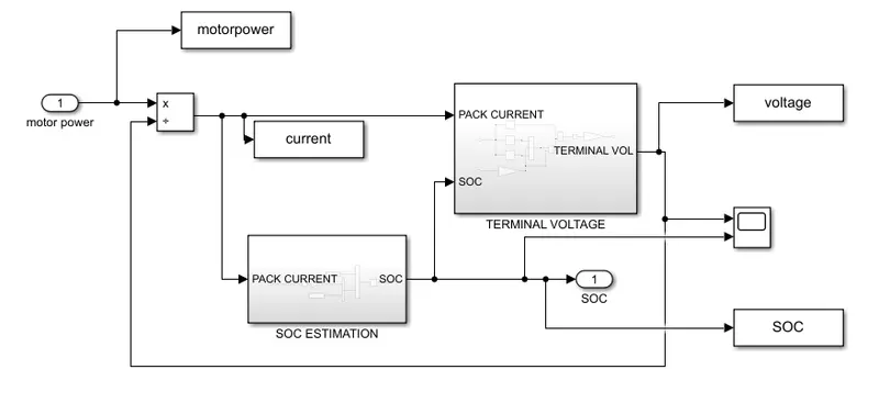
motor power is given as input and when is power is divided by voltage it gives the current.

soc block

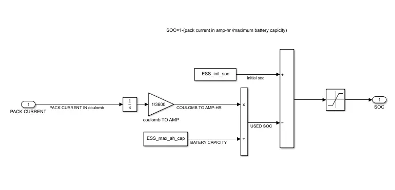
inside soc block first we are integrating the value of pack current which is in coulomb and with gain block we multiply it to convert into ahm-hr

soc= initial state of charge -used state of charge

used state of charge=pack current in amp-hr/maximum battery capicity (in ahm-hr)

this values are been saturated with upper limit 1 and lower limit 0

why this ( because we have given the maximum value in ESS SOC start from 0 end to 1)

terminal voltage

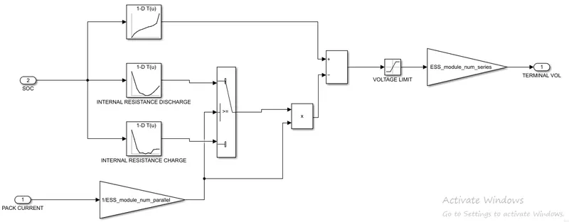
inside of terminal voltage bolck

we providing the input value in 1d lookup table for open curcuit voltage, internal resistance discharge , internal resistance charge and parall num module.

switch which checkes those values and pass further to calculate terminal voltage.

TRANSMISSION

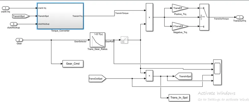
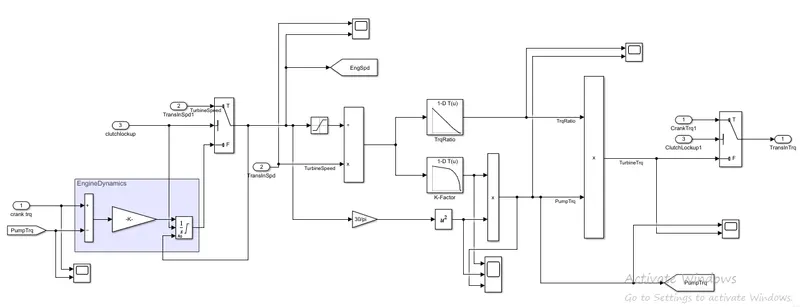
in engine dynamic gain block em inertia is added because both are coupled together. with the help of clutch lock up we are locking the torque convertor when the values are not similar..

PROCESSING CODE

%% Skill-Lync -> Hybrid Drives Development
% Project 2 - P1 hybrid Vehicle Model
% By - RITIK SONKAMBLE

%% Renaming variables
Time = tout;
Acc_Pdl = Acc_Pdl;          % Accelerator pedal [%]
Brk_Pdl = Brk_Pdl;          % Brake pedal [%]
Gear_Cmd = Gear_Cmd;        % Transmission gear
Trans_In_Spd = Trans_In_Spd*30/pi;  % Transmission input speed [rpm]
Trans_Out_Spd = Trans_Out_Spd*30/pi;% Transmission output speed [rpm]
Eng_Trq = Eng_Trq;          % Engine brake torque [Nm]
Eng_Spd = Eng_Spd*30/pi;    % Engine speed [rpm]
Eng_Fuel_Consump = Eng_Fuel_Consumption;    % Engine fuel consumption [g]
Veh_Dist = Veh_Dist/1000;   % Distance traveled by vehicle [km]
Veh_Spd = Veh_Spd*18/5;     % Vehicle speed [kmph]
WheelSpd=WheelSpd;            % wheel speed [rpm]
Eng_Fuel_rate=Eng_Fuel_Rate;
MOTORSPEED=motorspeed;
MOTORTORQUE=motortorque;
CURRENT=current;
VOLTAGE=voltage;
SOC=SOC;
MOTORPOWER=motorpower;
%% Data Analysis
Eng_Pwr = Eng_Spd.*pi./30.*Eng_Trq./1000;   % Engine brake power [kW]
rho_petrol = 0.7197;                    % Density of petrol [kg/L]
kmpl = Veh_Dist(end)/(Eng_Fuel_Consump(end)/1000/rho_petrol)    % Fuel economy [kmpl] 

%% TIME TRACT FOR ENGINE
figure(1)
hold on
grid on
plot(Time,Trans_In_Spd, 'linewidth', 1, 'Color', 'black')
plot(Time,Trans_Out_Spd, 'linewidth', 1, 'Color', 'red')
plot(Time,WheelSpd, 'linewidth', 1, 'Color', 'green')
xlabel('time [s]')
ylabel('speed [rpm]')
xlim([0, Time(end)]);
ylim([0, 6000]);
legend('Trans In Spd','Trans Out Spd','WheelSpd')
%% Plotting torque ,power,fuel rate,fuel consumption
figure(2)
subplot(4,1,1)
grid on
plot(Time, Eng_Trq, 'linewidth', 1, 'Color', 'black');
xlabel('time [s]')
ylabel('engine torque [Nm]')
xlim([0, Time(end)]);
subplot(4,1,2)
grid on
plot(Time, Eng_Pwr, 'linewidth', 1, 'Color', 'blue');
xlabel('time [s]')
ylabel('engine power [Nm]')
xlim([0, Time(end)]);
subplot(4,1,3)
grid on
plot(Time,Eng_Fuel_rate, 'linewidth', 1, 'Color', 'green');
xlim([0, Time(end)]);
xlabel('Time [s]');
ylabel('engine fuel rate');
subplot(4,1,4)
grid on
plot(Time,Eng_Fuel_Consump, 'linewidth', 1, 'Color', 'red');
xlim([0, Time(end)]);
xlabel('Time [s]');
ylabel('engine fuel consumption');
%% Plotting vehicle characteristics time trace
figure(3)
subplot(4,1,1)
hold on
grid on
plot(Time, Acc_Pdl, 'linewidth', 1, 'Color', 'black');
plot(Time, Brk_Pdl, 'linewidth', 1, 'Color', 'red');
ylabel('Pedal [%]')
xlim([0, Time(end)]);
legend('Accel','Brake');
subplot(4,1,2)
hold on
grid on
plot(Time, Gear_Cmd, 'linewidth', 1, 'Color', 'black');
xlim([0, Time(end)]);
xlabel('Time [s]');
ylabel('Gear');
subplot(4,1,3)
hold on
grid on
plot(cyc_time,(cyc_vel.*(18./5)), 'linewidth', 1, 'Color', 'black');
plot(Time, Veh_Spd, 'linewidth', 1, 'Color', 'red');
ylabel('velocity')
xlabel('Time [s]');
xlim([0, Time(end)]);
legend('desired speed','Actual speed');
subplot(4,1,4)
hold on
grid on
plot(Time, Veh_Dist, 'linewidth', 1, 'Color', 'black');
xlim([0, Time(end)]);
xlabel('Time [s]');
ylabel('distance [km]');

%% Plotting engine operating points on engine fuel map
figure('Name','Engine Operating Points');
hold on
grid on
title('Engine Operating Points','fontsize',12);
p1=plot(Eng_map_spd*30/pi,Eng_max_trq,'linewidth',2,'color','r');
p2=line([Eng_map_spd(end)*30/pi Eng_map_spd(end)*30/pi],[0 Eng_max_trq(end)]);
set(p2,'linewidth',1,'linestyle','--','color','k');
p3=line([Eng_map_spd(1)*30/pi Eng_map_spd(1)*30/pi],[0 Eng_max_trq(1)]);
set(p3,'linewidth',1,'linestyle','--','color','k');
[c,h] = contour(Eng_map_spd'*30/pi,Eng_map_trq,Eng_fuel_map');
clabel(c,h);
xlabel('Engine Speed [rpm]');
ylabel('Engine Torque [Nm]');
title('Engine Fuel Consumption Map [g/s]');
p4 = plot(Eng_Spd,Eng_Trq,'.','color','k');
legend([p1 p4],{'Max Curve','Operating Points'});
axis([Eng_map_spd(1)*30/pi Eng_map_spd(end)*30/pi 0 Eng_map_trq(end)]);
%% Plot motor speed, torque, motor input power using subplots.
figure(5)
subplot(3,1,1)
grid on
plot(Time,MOTORSPEED,'linewidth', 1, 'Color', 'black')
xlabel('time [s]')
ylabel('MOTOR SPEED [rpm]')
xlim([0, Time(end)]);
subplot(3,1,2)
grid on
plot(Time,MOTORTORQUE,'linewidth', 1, 'Color', 'blue')
xlabel('time [s]')
ylabel('MOTOR TORQUE [Nm]')
xlim([0, Time(end)]);
subplot(3,1,3)
grid on
plot(Time, MOTORPOWER,'linewidth', 1, 'Color', 'red')
xlabel('time [s]')
ylabel('motorpower ')
xlim([0, Time(end)]);


%% Plot pack voltage, current and SoC using subplots.
figure(6)
subplot(3,1,1)
grid on
plot(Time,VOLTAGE,'linewidth', 1, 'Color', 'black')
xlabel('time [s]')
ylabel('VOLTAGE [V]')
xlim([0, Time(end)]);
subplot(3,1,2)
grid on
plot(Time,CURRENT,'linewidth', 1, 'Color', 'blue')
xlabel('time [s]')
ylabel('CURRENT [A]')
xlim([0, Time(end)]);
subplot(3,1,3)
grid on
plot(Time,SOC,'linewidth', 1, 'Color', 'red')
xlabel('time [s]')
ylabel('SOC [%] ')
xlim([0, Time(end)]);

%% Plotting motor operating points 
figure('Name','motor operating points');
hold on
grid on
title('motor operating points','fontsize',12);
p1=plot(EM_map_spd*30/pi,EM_max_trq,'linewidth',2,'color','r');
p2=line([EM_map_spd(end)*30/pi EM_map_spd(end)*30/pi],[0 EM_map_trq(end)]);
set(p2,'linewidth',1,'linestyle','--','color','k');
p3=line([EM_map_spd(1)*30/pi EM_map_spd(1)*30/pi],[0 EM_max_trq(1)]);
set(p3,'linewidth',1,'linestyle','--','color','k');
[c,h] = contour(EM_map_spd'*30/pi,EM_map_trq,EM_inpwr_map');
clabel(c,h);
xlabel('motor Speed [rpm]');
ylabel('motor Torque [Nm]');
title('motor input power Map [g/s]');
p4 = plot(MOTORSPEED,MOTORTORQUE,'.','color','k');
legend([p1 p4],{'Max Curve','Operating Points'});
axis([EM_map_spd(1)*30/pi EM_map_spd(end)*30/pi 0 EM_map_trq(end)]);

data taken from the the simulink model and plots are coded

PLOTS

1]Plot the time trace for engine, transmission input, transmission output and wheel speed on one plot.

UDDS DRIVE CYCLE

HWFET DRIVE CYCLE

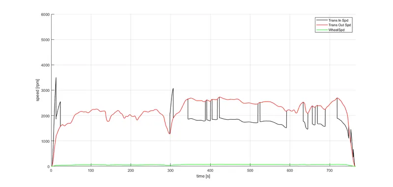
there is more fluctuation in speed .means transmisson speed is decreasing to zero in every few time which cause less out energy generation .as compaire to figure 2 we can see that there is less fluctuation means transmission speed is very low to zero for long period of time which produce more energy

2] Plot engine torque, engine power, fuel rate and fuel consumption using subplots.

UDDS CYCLE

HWFET CYCLE

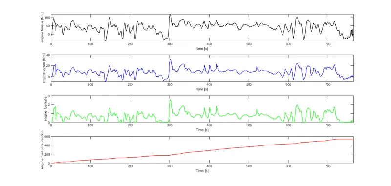
we can see the engine torque, engine power, fuel rate is directly proportional to each other . which means as engine power is increased the torque is also increased and at time fuel rate is also increase the main difference between figure 1and 2 OF ABOVE FIGURE is fluctuation due to instant increase and decrease in power,torque ,fuel rate. due to the driving condition.

3] Plot accelerator and brake pedal, gear command, vehicle desired and actual speed, vehicle distance using subplots.

UDDS CYCLE

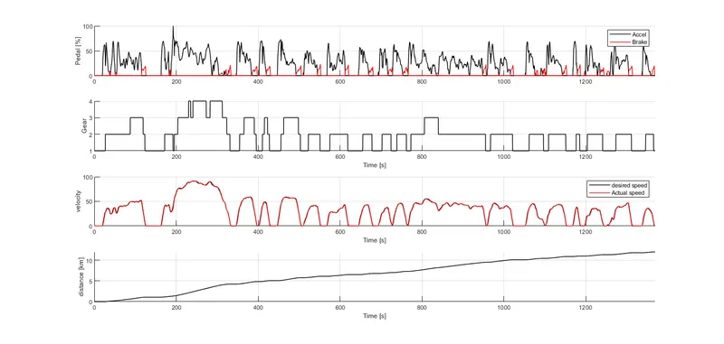
HWFET CYCLE

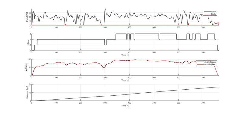
the gear is not constant for long period we will recieve less velocity where as in figure HWFET the gear is constant for long period means velocity is also increasing due to which there is less pedeling and cause less power loss. by looking at the graph UDDS and HWFET we can identify that vehical is stopped multipal time in a given distance due to zero velocity at multipal time for UDDS cycle where as in HWFET cycle no vehical stop multipal time in given diastance due to gradually increasing and decreasing in velocity without making it zero.

4] Plot the engine operating points on the engine fuel map.

UDDS CYCLE

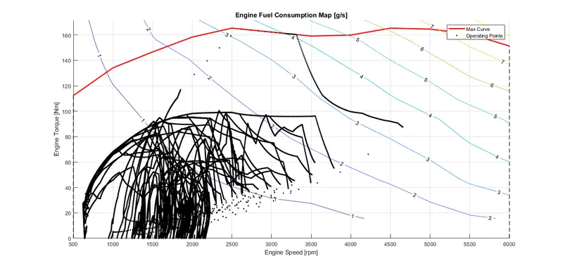
HWFET CYCLE

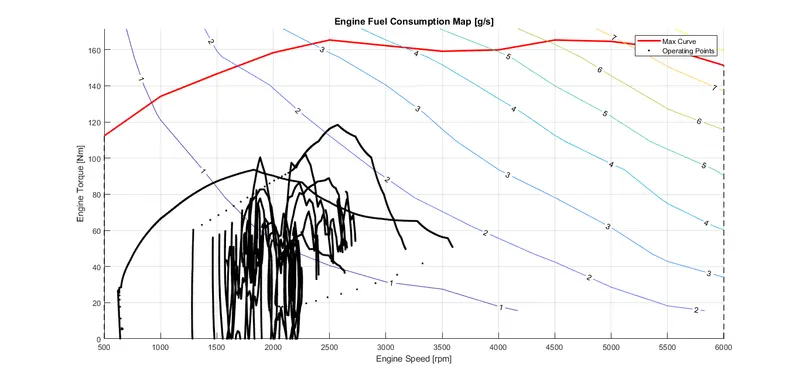
ENGINE OPERATING POINT OF UDDS CYCLE are at 46000 rpm to 160 nm torque where ad hwfet cycle is showing less of it.

5}Plot motor speed, torque, motor input power using subplots.

UDDS CYCLE

HWFET CYCLE

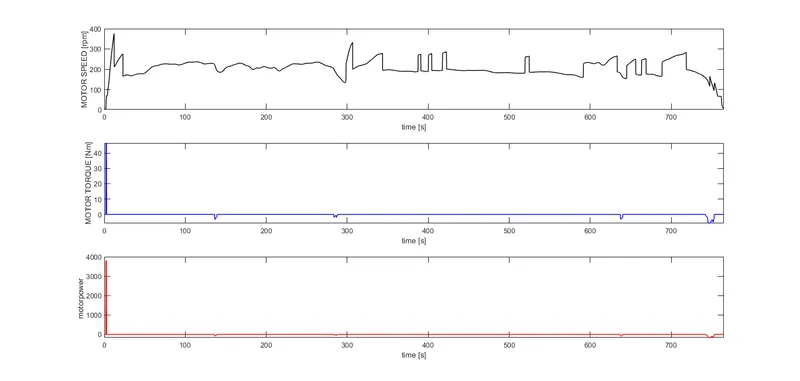
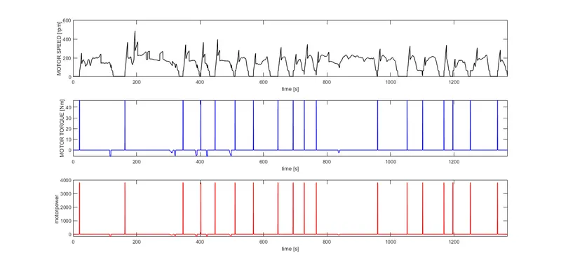
more fluctuation is there isin UDDS CYCLE THEN HWFET BECAUSE UDDS MANY START AND BREAK CONDITION DUE TO ITS NATURE the function of our model is to rotate crank and which is more in UDDS cycle as compaie to hdfet.

the motor power and torque is high at begning then goes to zero because continous fluctuion is there.

6] Plot pack voltage, current and SoC using subplots.

UDDS CYCLE

HWFET CYCLE

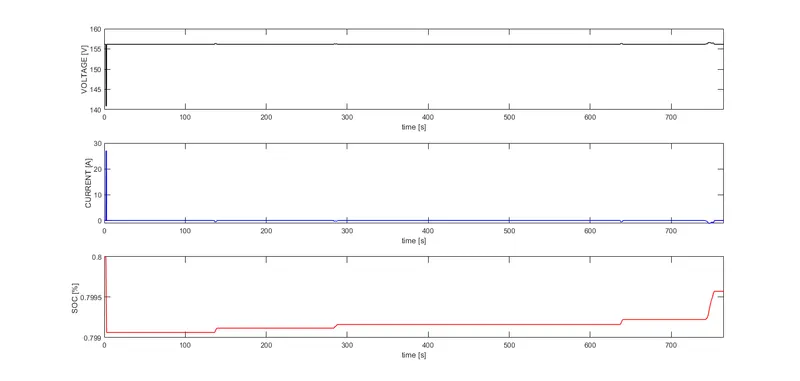
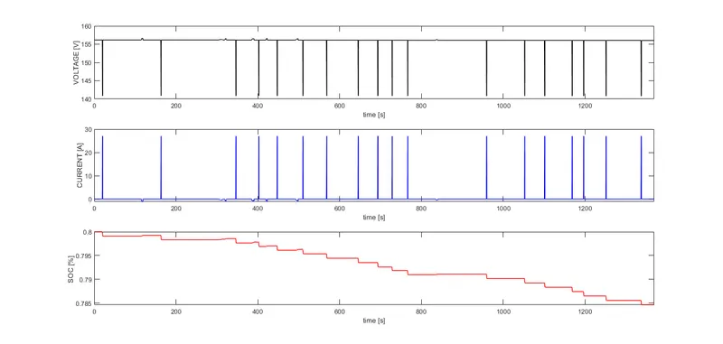
in udds cycle we can see when voltage is dropping current is increasing and when current is increasing voltage is droping because ther are directly proportion to each other.

soc is dropping in udds cycle because there is many stop and srtart in udds cycle means moter is to be on and off many time which causes soc decrease and less charging .

where as in hwfet cycle less time moter is turned on which causes battery charge more.soc(state of charge)

7] Plot the motor operating points on the motor input power map, with the motor max motoring and generating torque curves.

UDDS CYCLE

HWFET CYCLE

Tabulate the fuel economy numbers (kmpl) for UDDS and HWFET cycle. Compare these numbers with the baseline numbers for conventional vehicle model from

Project 1.

values from project 2

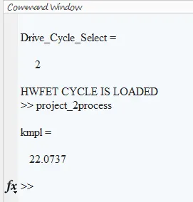
values from project 1

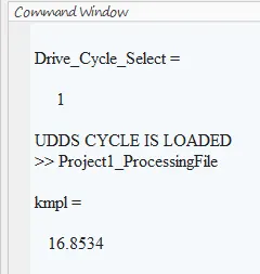
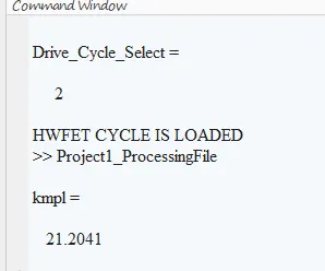
fuel economic number is in HWFET cycle is higher because ther is low pealing which cause low energy loss which cause less fuel consumption where as as compaire to UDDS cycle there is more pedeling means more energy loss due to loss which cause more fuel consumption .

as we can se the result that by using p1 hybrid we are getting more fuel consumption rate as compair to conventional vehical (project1).

THANK YOU