Week - 9 Material Modeling from Raw Data

MATERIAL MODELING FROM RAW DATA USING LS-DYNA

INTRODUCTION:

The LS-DYNA software's huge library of material models for a wide range of materials is a key feature. To apply these material models, model coefficients or parameters must be obtained, where material attributes are translated into the values required by the constitutive equations. While some models are simple, the majority are complicated and require some knowledge to understand how to extract model parameters. The material attributes are obtained by running certain tests on the target material. The input is then converted through a series of steps to produce the values or material parameters that feed the material model.
When these characteristics are appropriately recognized, the material model uses them to numerically re-create the intended material behaviors for use in software computations. Proper parameter identification is therefore critical to the simulation's performance; otherwise, severe error or failure can occur. Materials models and simulation tools are required to eliminate trial-and-error loops during the development of materials, components, and manufacturing processes, to illustrate complex load scenarios, and to make reliable predictions of the behavior of existing and developing materials and components.

The material model is provided as a mask over the underlying data in the CAE Modeller user interface so that the user may judge the goodness of fit between the model and raw data. In the case of the MAT_024 material model, for example, the selected equivalent stress v. plastic strain data points are back-calculated to stress-strain, allowing everything to be evaluated in the context of the known stress-strain curves.

The measurement of relevant material data is a critical step prior to the parameter identification process. This necessitates a thorough grasp of the material model's data requirements, the material's behavior, and the physical constraints of the testing procedure.
In most cases, the material model documentation and software specify the input data required for the material model. The problems associated with acquiring the correct data increase as the materials become more complicated.

The materials modeled by the material model are frequently complicated and multivariate in character, necessitating some type of approximation to correlate real life to mathematics. These variables can have an effect on the simulation's realism. Testing is frequently constrained by physical constraints, such as the inability to carry out the tests in the manner predicted by the model theory. Writing the output file is a mechanical process that entails writing the data in the correct format. All necessary options and flags must be set correctly. To capture all of the needed data, LS-DYNA's file format cascades using mixes of tables and curves. If the file is appropriately written, the material parameters will be read into LS-DYNA. Validation is the process of comparing the material model to the simulation. It has three degrees of difficulty. The unit element test simply ensures that the model does not produce non-physical outcomes by running it against a single finite element. The goal of closed-loop validation is to replicate the original test that generated the material model. In the MAT-24 scenario, tensile testing would be simulated to see if the original stress-strain curves were replicated. The most complex validation method is open-loop validation, in which an alternate or multi-mode experiment is compared to a simulation.

AIM:

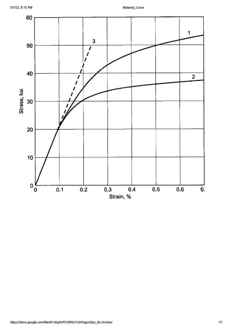
Use the diagram of the true stress-strain curve of graphite iron casting. Two curves are there for different material structures. Select one of these and use the data to generate a MAT_024 or MAT_018 material model, which must then be validated.

The primary objectives for this assignment are as follows:

1. Extract the data from the diagram
2. Clean the data and visually confirm that it matches the original data and the elastic modulus is 20.9E+06 psi.
3. Convert the data to (kg-mm-ms) unit system
4. Process the data and create the material as demonstrated
5. Use the material model with a dogbone specimen and validate the same.

EXPLANATION:

• The input values of corresponding stress and strains from the given graph image are calculated by plotting points using a data digitizer tool prior to solving and post-processing.

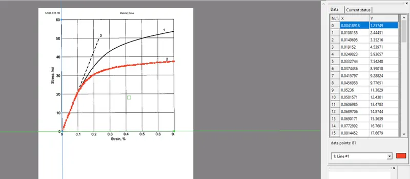
• The raw data is computed in a tabular format and generated in the form of a True stress-strain curve. The conversion of engineering to true stress/strains is done using the formulas ascribed:

True strain = ln(1 + engineering strain) where ln designates the natural log

True stress = (engineering stress) * exp(true strain) = (engineering stress) * (1 + engineering strain) where exp(true strain) is 2.71 raised to the power of (true strain).

True Strain(%) True Stress(ksi)

4.19E-03 1.26E+00

1.08E-02 2.44E+00

1.50E-02 3.35E+00

1.92E-02 4.54E+00

2.50E-02 5.94E+00

3.33E-02 7.54E+00

3.74E-02 8.59E+00

4.16E-02 9.29E+00

4.57E-02 9.78E+00

5.24E-02 1.14E+01

5.82E-02 1.24E+01

6.07E-02 1.35E+01

6.90E-02 1.49E+01

6.90E-02 1.54E+01

7.73E-02 1.68E+01

8.14E-02 1.77E+01

8.56E-02 1.85E+01

8.97E-02 1.91E+01

9.14E-02 1.98E+01

9.56E-02 2.06E+01

1.04E-01 2.16E+01

1.06E-01 2.22E+01

1.15E-01 2.29E+01

1.19E-01 2.34E+01

1.24E-01 2.44E+01

1.31E-01 2.51E+01

1.35E-01 2.55E+01

1.41E-01 2.60E+01

1.45E-01 2.69E+01

1.52E-01 2.72E+01

1.56E-01 2.74E+01

1.60E-01 2.78E+01

1.68E-01 2.83E+01

1.72E-01 2.86E+01

1.78E-01 2.90E+01

1.82E-01 2.95E+01

1.93E-01 3.00E+01

2.02E-01 3.06E+01

2.09E-01 3.09E+01

2.19E-01 3.14E+01

2.25E-01 3.14E+01

2.33E-01 3.17E+01

2.43E-01 3.21E+01

2.50E-01 3.23E+01

2.55E-01 3.24E+01

2.64E-01 3.28E+01

2.72E-01 3.30E+01

2.82E-01 3.31E+01

2.92E-01 3.33E+01

3.07E-01 3.37E+01

3.19E-01 3.40E+01

3.29E-01 3.42E+01

3.41E-01 3.45E+01

3.56E-01 3.45E+01

3.64E-01 3.47E+01

3.76E-01 3.49E+01

3.86E-01 3.48E+01

3.94E-01 3.51E+01

4.05E-01 3.52E+01

4.13E-01 3.54E+01

4.25E-01 3.54E+01

4.41E-01 3.54E+01

4.51E-01 3.55E+01

4.62E-01 3.55E+01

4.75E-01 3.59E+01

4.94E-01 3.59E+01

5.06E-01 3.61E+01

5.16E-01 3.61E+01

5.33E-01 3.62E+01

5.53E-01 3.65E+01

5.63E-01 3.65E+01

5.80E-01 3.65E+01

5.96E-01 3.69E+01

6.12E-01 3.69E+01

6.18E-01 3.69E+01

6.38E-01 3.71E+01

6.49E-01 3.71E+01

6.63E-01 3.71E+01

6.73E-01 3.72E+01

6.95E-01 3.74E+01

7.02E-01 3.74E+01

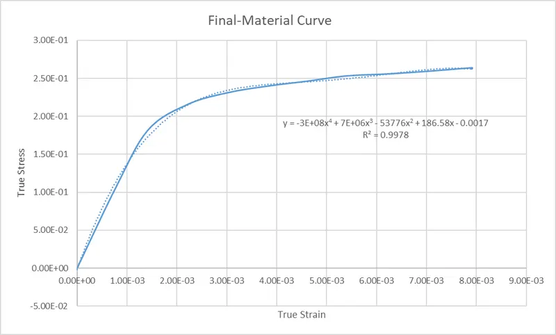
• The original material curve of the graphite iron casting/ductile iron is displayed below with the trendline precision. The coefficient of determination, or R², is a metric that indicates the quality of fit of a model. In the context of regression, it is a statistical measure of how closely the line of regression approximates the real data. The equation of the line developed from the curve is attached to it also.

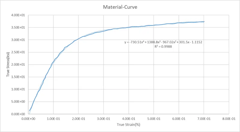
• The unit system allocated for this assignment is in (kg-mm-ms) so we convert the stress and stresses accordingly.
• For True strain, we remove the percentage by using the formula for the first value and likewise for others as 4.19E-03 x 100
• Similarly for true stress, we convert ksi to GPa viz. 1.26E+00 x 0.0068947573 (1 ksi or kilopound force per square inch = 0.00689476 GPa or Giga pascal)

True Strain True Stress(GPa)

4.19E-05 8.67E-03

1.08E-04 1.69E-02

1.50E-04 2.31E-02

1.92E-04 3.13E-02

2.50E-04 4.09E-02

3.33E-04 5.20E-02

3.74E-04 5.92E-02

4.16E-04 6.40E-02

4.57E-04 6.74E-02

5.24E-04 7.85E-02

5.82E-04 8.57E-02

6.07E-04 9.29E-02

6.90E-04 1.03E-01

6.90E-04 1.06E-01

7.73E-04 1.16E-01

8.14E-04 1.22E-01

8.56E-04 1.28E-01

8.97E-04 1.31E-01

9.14E-04 1.36E-01

9.56E-04 1.42E-01

1.04E-03 1.49E-01

1.06E-03 1.53E-01

1.15E-03 1.58E-01

1.19E-03 1.61E-01

1.24E-03 1.68E-01

1.31E-03 1.73E-01

1.35E-03 1.76E-01

1.41E-03 1.80E-01

1.45E-03 1.85E-01

1.52E-03 1.88E-01

1.56E-03 1.89E-01

1.60E-03 1.92E-01

1.68E-03 1.95E-01

1.72E-03 1.97E-01

1.78E-03 2.00E-01

1.82E-03 2.04E-01

1.93E-03 2.07E-01

2.02E-03 2.11E-01

2.09E-03 2.13E-01

2.19E-03 2.17E-01

2.25E-03 2.17E-01

2.33E-03 2.19E-01

2.43E-03 2.21E-01

2.50E-03 2.23E-01

2.55E-03 2.24E-01

2.64E-03 2.26E-01

2.72E-03 2.27E-01

2.82E-03 2.28E-01

2.92E-03 2.30E-01

3.07E-03 2.32E-01

3.19E-03 2.35E-01

3.29E-03 2.36E-01

3.41E-03 2.38E-01

3.56E-03 2.38E-01

3.64E-03 2.39E-01

3.76E-03 2.40E-01

3.86E-03 2.40E-01

3.94E-03 2.42E-01

4.05E-03 2.43E-01

4.13E-03 2.44E-01

4.25E-03 2.44E-01

4.41E-03 2.44E-01

4.51E-03 2.45E-01

4.62E-03 2.45E-01

4.75E-03 2.47E-01

4.94E-03 2.47E-01

5.06E-03 2.49E-01

5.16E-03 2.49E-01

5.33E-03 2.50E-01

5.53E-03 2.52E-01

5.63E-03 2.52E-01

5.80E-03 2.52E-01

5.96E-03 2.54E-01

6.12E-03 2.54E-01

6.18E-03 2.54E-01

6.38E-03 2.56E-01

6.49E-03 2.56E-01

6.63E-03 2.56E-01

6.73E-03 2.57E-01

6.95E-03 2.58E-01

7.02E-03 2.58E-01

• Nevertheless, we need to plot effective true strain and effective/true stress for the material modeling process so we will use the corresponding formula for the stress and strains obtained as

effective plastic strain (input value) = total true strain - true stress/E

• E = 20.9E+06 psi = 144.1 GPa (The value of E is given which is converted by the allocated unit system)

Effective Plastic Strain Effective/ True Stress(Gpa)

-1.83E-05 0.008670059

-8.82E-06 0.016852935

-1.07E-05 0.023112309

-2.57E-05 0.031300231

-3.42E-05 0.040931201

-2.81E-05 0.052003536

-3.66E-05 0.059227184

-2.86E-05 0.064040146

-1.08E-05 0.067406696

-2.10E-05 0.078482396

-1.32E-05 0.08570268

-3.79E-05 0.092929691

-2.20E-05 0.102555615

-4.49E-05 0.105930575

-2.90E-05 0.115556499

-3.09E-05 0.121815872

-2.95E-05 0.127593109

-1.50E-05 0.131441796

-3.15E-05 0.136259804

-3.01E-05 0.14203704

2.24E-06 0.149252279

4.61E-07 0.15310433

4.92E-05 0.157908883

6.70E-05 0.161275433

7.48E-05 0.168495717

1.07E-04 0.173303634

1.32E-04 0.17570591

1.62E-04 0.179551234

1.64E-04 0.18532847

2.13E-04 0.187725701

2.44E-04 0.189163703

2.68E-04 0.19156598

3.26E-04 0.194924121

3.51E-04 0.197326397

3.91E-04 0.19972531

4.06E-04 0.203573997

4.89E-04 0.206927093

5.61E-04 0.210764008

6.09E-04 0.213161238

6.84E-04 0.216516016

7.49E-04 0.216502561

8.15E-04 0.218896428

8.96E-04 0.221286931

9.51E-04 0.222719887

1.00E-03 0.223672389

1.07E-03 0.226066256

1.14E-03 0.227495848

1.24E-03 0.228438258

1.33E-03 0.229864487

1.46E-03 0.232244899

1.56E-03 0.234630357

1.65E-03 0.235574448

1.76E-03 0.237959906

1.91E-03 0.237929632

1.98E-03 0.239359225

2.09E-03 0.240298271

2.19E-03 0.240278089

2.26E-03 0.241707681

2.36E-03 0.242650091

2.43E-03 0.244079684

2.56E-03 0.244054456

2.72E-03 0.244020818

2.81E-03 0.24496491

2.92E-03 0.244943046

3.04E-03 0.24732514

3.23E-03 0.247286456

3.34E-03 0.24870764

3.44E-03 0.248687457

3.59E-03 0.249618094

3.78E-03 0.251986733

3.89E-03 0.251964869

4.05E-03 0.251931231

4.20E-03 0.254308279

4.36E-03 0.254274642

4.42E-03 0.254262869

4.61E-03 0.255667233

4.72E-03 0.255645369

4.85E-03 0.255616777

4.95E-03 0.256559187

5.16E-03 0.257960188

5.23E-03 0.257946733

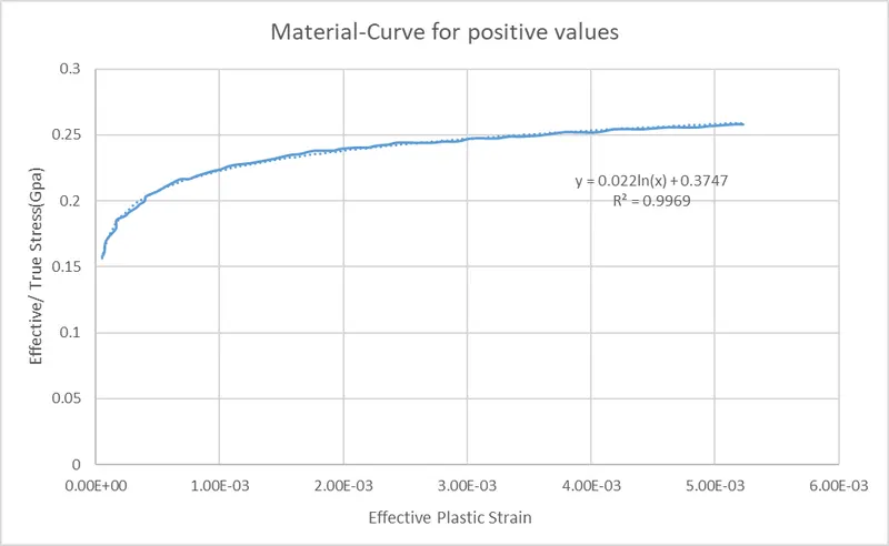
• The graphs we generated have a lot of noise(not smooth) so in order to get clean data we take positive and advancing values with equidistant spaces between two intervals by following the particular formula as follows:

Input-Effective Plastic Strain= First Effective plastic strain positive value + Common difference

Common difference = (Last positive Effective Plastic strain - First positive Effective plastic strain)/ Number of values

Input-Effective/ True Stress(Gpa) = 0.022*LN(First positive Effective plastic strain)+0.3747

• The respective consecutive values are placed in the formula instead of the first positive effective plastic strain values in order to find out other unknown 60 values.

Input-Effective Plastic Strain Input-Effective/ True Stress(Gpa) Common difference

4.60791E-07 0.053712937 8.71456E-05

8.76063E-05 0.169161544

0.000174752 0.184352848

0.000261897 0.193253735

0.000349043 0.199573062

0.000436189 0.20447641

0.000523334 0.208483611

0.00061048 0.211872158

0.000697625 0.214807773

0.000784771 0.217397385

0.000871916 0.219714025

0.000959062 0.221809792

0.001046207 0.223723161

0.001133353 0.225483355

0.001220499 0.227113092

0.001307644 0.228630381

0.00139479 0.230049744

0.001481935 0.231383058

0.001569081 0.232640163

0.001656226 0.233829302

0.001743372 0.234957449

0.001830517 0.236030555

0.001917663 0.237053744

0.002004809 0.238031453

0.002091954 0.238967554

0.0021791 0.239865444

0.002266245 0.24072812

0.002353391 0.241558242

0.002440536 0.242358176

0.002527682 0.243130042

0.002614827 0.243875743

0.002701973 0.244596994

0.002789119 0.245295348

0.002876264 0.245972214

0.00296341 0.246628876

0.003050555 0.247266504

0.003137701 0.247886171

0.003224846 0.248488861

0.003311992 0.249075479

0.003399137 0.249646862

0.003486283 0.250203779

0.003573429 0.250746945

0.003660574 0.251277024

0.00374772 0.251794631

0.003834865 0.252300339

0.003922011 0.252794683

0.004009156 0.253278162

0.004096302 0.253751245

0.004183447 0.254214369

0.004270593 0.254667943

0.004357739 0.255112355

0.004444884 0.255547968

0.00453203 0.255975122

0.004619175 0.25639414

0.004706321 0.256805326

0.004793466 0.257208968

0.004880612 0.257605337

0.004967758 0.257994692

0.005054903 0.258377275

0.005142049 0.258753318

0.005229194 0.259123042

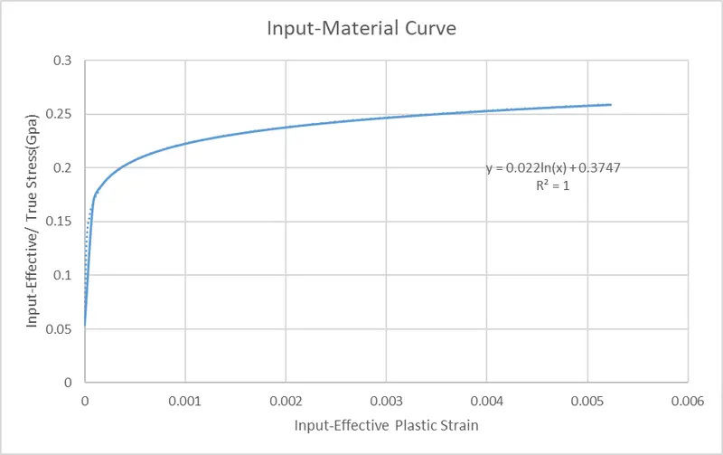
• Since we facilitated the stress-strain graph for the ductile iron material so we will proceed with the post-processing phase in LS-Dyna.
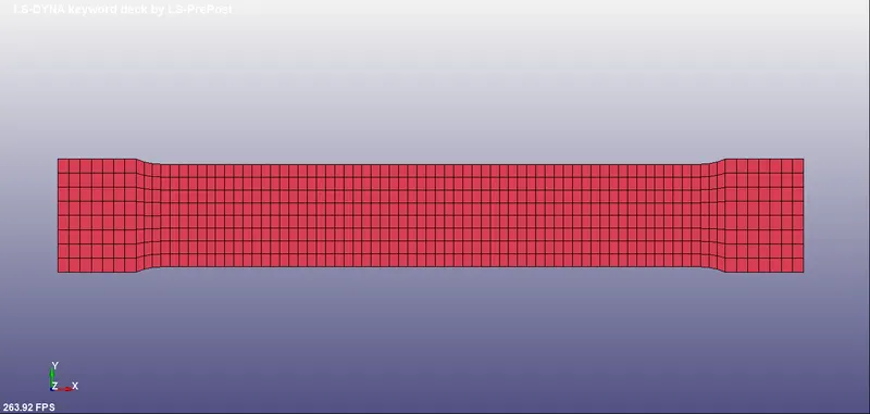
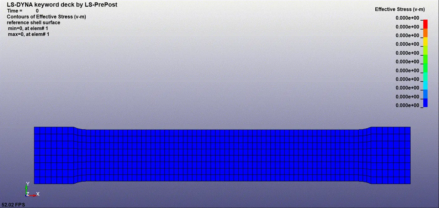
• The given model namely dog-bone comprised of a shell element layer is imported as a keyword file.

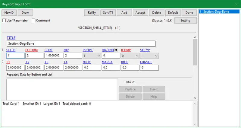
• The mandatory cards like section shell card is inputted with Elform 2 and thickness as 2mm.

• Mat_024 card is employed for this type of analysis in this task with specific parameters. The material here used is Graphite-Iron casting also known as ductile iron. Ductile iron, additionally referred to as nodular iron or spheroidal graphite iron, has a similar composition to grey iron, but the graphite nucleates as spherical particles (nodules) in ductile iron rather than as flakes after solidification. Ductile iron is not a single material, but rather a set of materials that may be manufactured with a variety of characteristics by manipulating their microstructure. Depending on the heat treatment, the matrix phase enclosing these particles is either pearlite or ferrite. Because ductile iron is stronger and more stress resistant than grey iron, even if it is more expensive owing to alloys, it may be the more cost-effective option because a lighter casting can fulfill the same purpose.
• The values of default quantities required for Mat_024 card are acquired from the type of material used i.e. ductile iron. However, we need to convert the default values with respect to the given unit system which is formulated as follows:

• Yield strength (SIGY) = 621

  = 621 x 0.2 (0.2% strain offset)

  = 124.2 MPa

  = 124.2/1000

  = 0.124 GPa

  Poisson’s ratio (PR) = 0.24

  Density (RO) = 7300 Kg/m³

  = 7300 x 10^-9 Kg/mm³

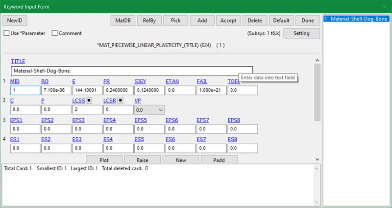
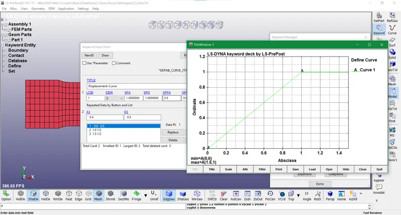
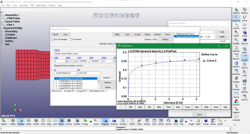
• The effective plastic stress-strain curve derived earlier is assigned in the LCSS of this material card. The displacement curve and stress-strain curve are generated in Define>Curve card as displayed below.

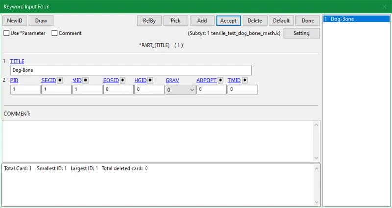
• The Section ID and Material ID are designated with a Part ID by creating a Part card.

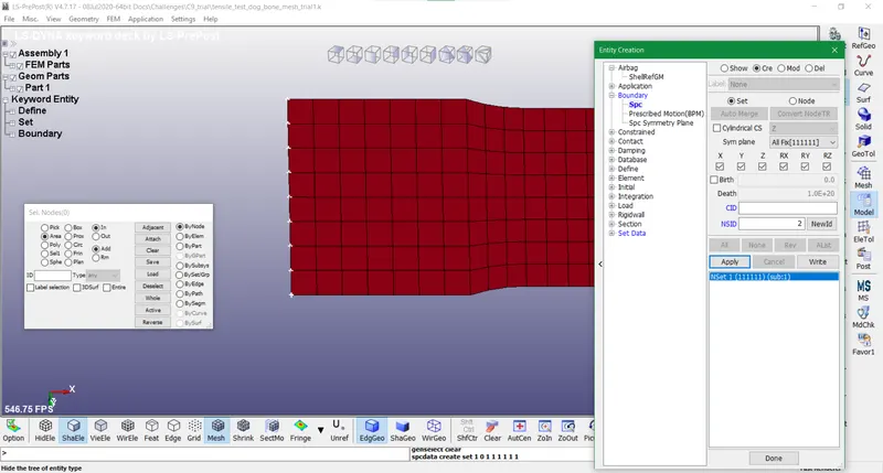
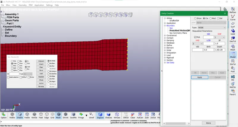
• Henceforth the type of scheme used for this simulation is implicit analysis so we create an SPC card on one side of the model with nodes constrained in all directions. Also prescribed motion in terms of displacement is attributed to the other side of the model in translational x direction only.

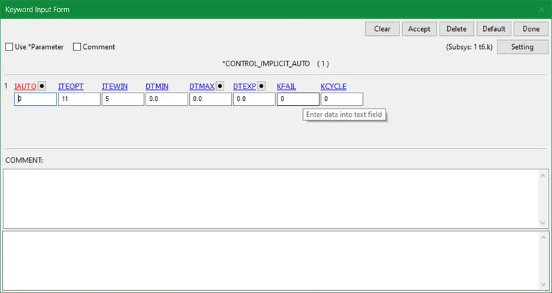
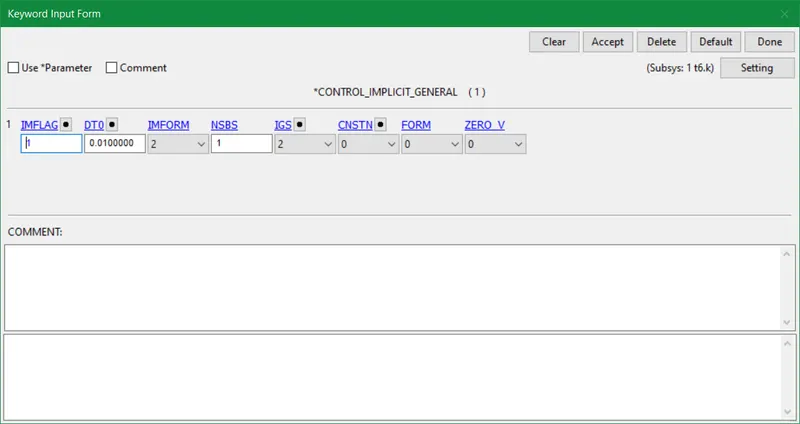
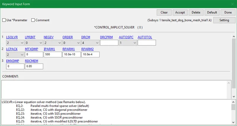
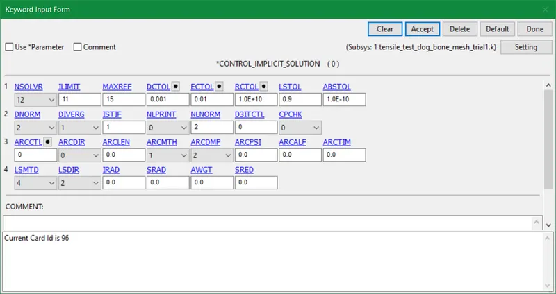
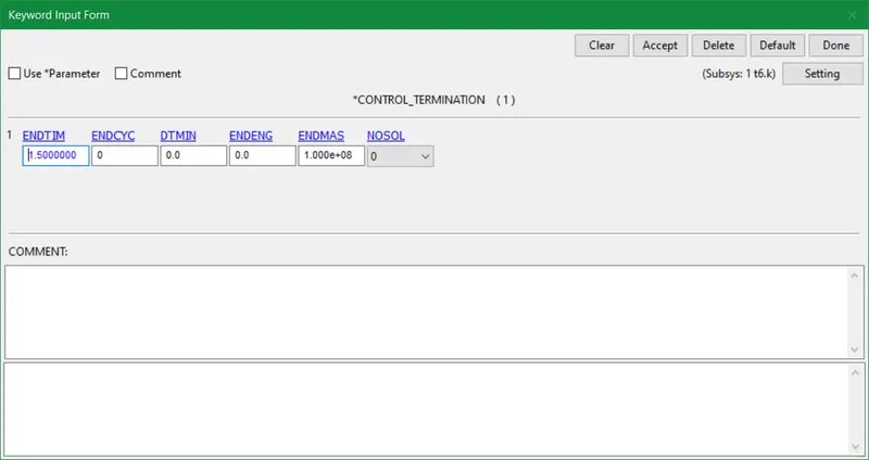
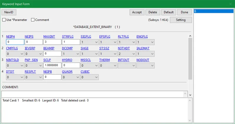
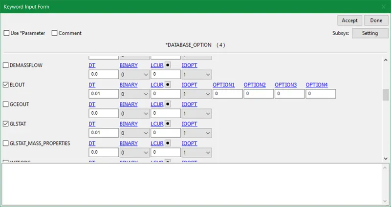
• The implicit cards and other mandatory cards like control termination, ASCII, and Database_Extent_Binary are allocated with specific and default values as per the calculations.

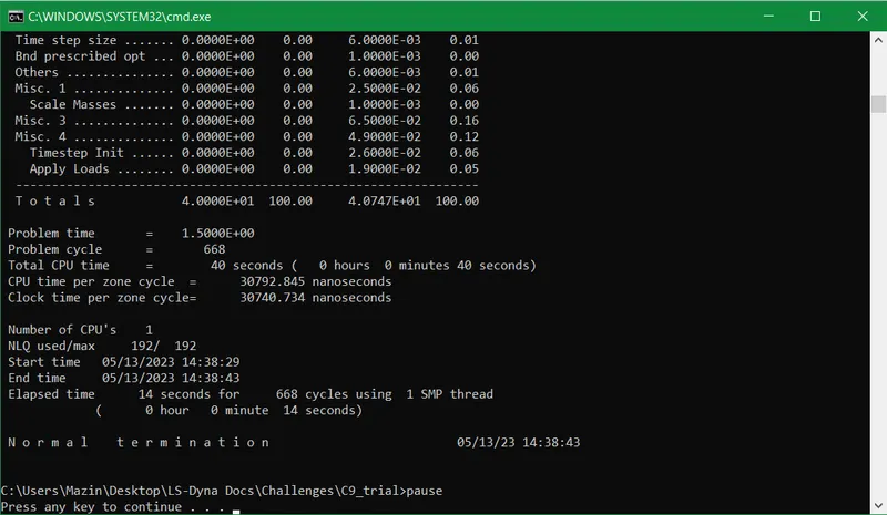
• Without further ado, we run the simulation and it gives normal termination results. The stress-strain curve is determined by a specific element in the model. In this case, we choose the 311th shell element in the middle of the dog-bone component.

• After several failures, we received the final material curve which is quite superimposing the original material curve as mentioned at the start.

CONCLUSION:

1. The simulated material curve of stress-strain values is achieved with sheer accuracy for the coefficient of determination w.r.t the original material curve.
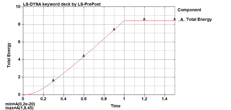
2. The total energy extracted is equal to the displacement curve given in this simulation and runs smoothly.
3. The stress and strain follow an elastic phase up to the yield point and then change to the plastic phase like the tensile test for ductile materials.
4. The failures of plotted results and calculations for effective plastic stress-strain are formulated and computed in the Excel files attached to this assignment.