2D ELEMENT FORMULATION USING RADIOSS

INTRODUCTION

The calculations and presumptions that guide the generation of displacements for various finite element types are known as element formulation in finite element analysis.

In FEA, elements are often classified as 1D, 2D, or 3D elements. They can be identified by their shapes, which include tetrahedral, triangular, quadrilateral, straight line, and many more. A line consisting of two nodes is the most basic component.

The displacement-based minimum principle is simply applied in the finite element formulation. The reinforcing beam and matrix material domain are discretized into triangular elements to achieve this.

The number of nodes on an element's edge is indicated by the element's order. The only nodes on first-order elements are found at the edges' corners. Mid-side nodes, which are located at various positions along the element edges, are also present in higher-order elements.

A collection of 1D elements is integrated into RADIOSS for use in FEA modelling. To determine the behaviour of a one-dimensional element, two nodes are connected linearly, and the element is then given constant cross-sectional properties. Truss elements, beam elements, and spring elements are the three common forms of one-dimensional elements that are available.

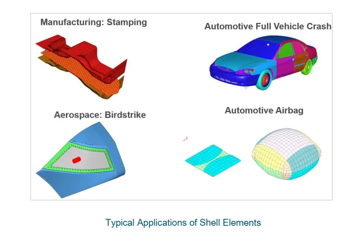
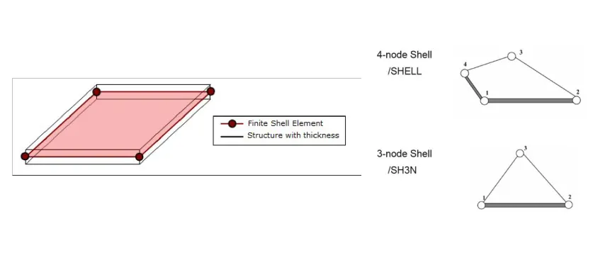
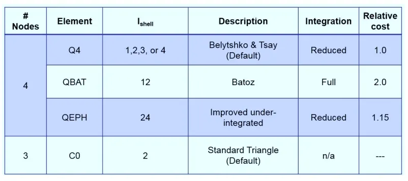
Shell elements are 2D planar, three or four-node elements with a constant thickness. They can be positioned in space and have a triangular or quadrilateral shape. They are commonly used to model several types of constructions, including aeroplane fuselage, automotive bodywork, ship hulls, and pressure vessels. There are six degrees of freedom available to shell elements since they support all translational and rotational degrees of freedom. The Mindlin-Reissner theory, which covers transverse shear deformation and applies to moderately thick and thin shells, is the foundation for RADIOSS shells. RADIOSS offers 4-noded shell elements that are both fully integrated and reduced.

Tetrahedral (4 faces), pentahedral (5 faces), pyramid (5 faces), and hexahedral (6 faces) elements are the accessible 3D solid elements. The number of nodes in brick or tetrahedral elements can vary, and solid elements can only support translational DOF.

Since all three dimensions are equivalent, they are used to model solid things when beam and shell elements are either not appropriate to model or cannot be used.

OBJECTIVES

Comparison of results with base simulation and improved shell element properties

1. Using the crash beam file from the previous assignment, change the run time to 55 ms.

2. Change the number of animation steps during simulation to a minimum of 25 and a maximum of 60.

3. Run the base simulation without any modification to element properties.

4. At the end of the simulation, do the energy error and mass error checks and determine whether the results would be acceptable.

5. If acceptable, Plot rigid wall forces, internal energy, hourglass energy, contact energy, and total energy of the simulations.

6. Change all the shell element's properties to recommended properties, save this as separate, rad files and run the simulation.

7. Follow steps 5 and 6.

8. Create a brief report comparing all the results from steps 5 and 6 for both simulations.

9. Comment whether there is any change in the results and why there is any change in the result.

Recommended properties:

Parameters		Comment
Ishell =24		QEPH 4 nodes shells are the best combination of cost and accuracy.
Ismstr=2		Full geometric nonlinearities (default)with possible small strain formulation activation in RADIOSS Engine.
Ish3n=2		Standard 3 noded shell (C0)with modification for large rotation(default)
N=5		Number of integration points is set to 5 for accuracy bending.
Ithick=1		Thickness change is taken into account for accuracy.
Iplas=1		Iterative plasticity for good accuracy.

PROCEDURE

BASE SIMULATION

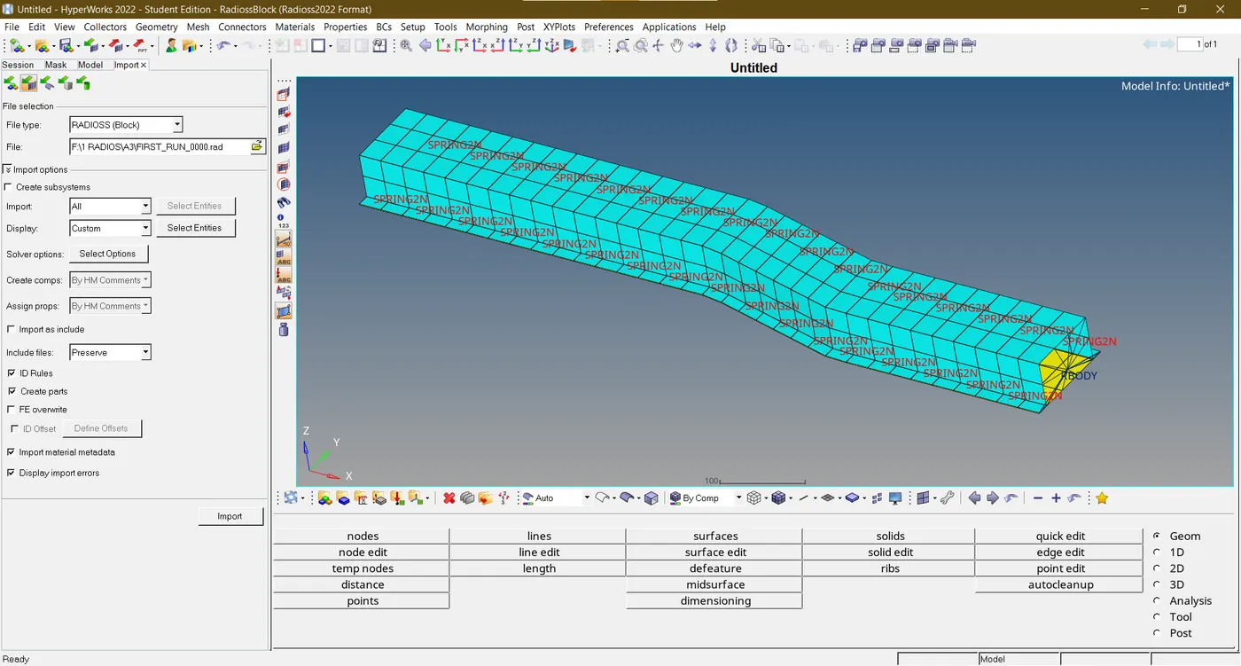
• In this assignment, the effect of shell formulations is studied and the nature of energies, mass error and other parameters is analyzed thoroughly. The given beam model is imported in the RADIOSS Solver deck as displayed below.

• In the ENG_RUN card, the termination or end time is registered as 55 ms.

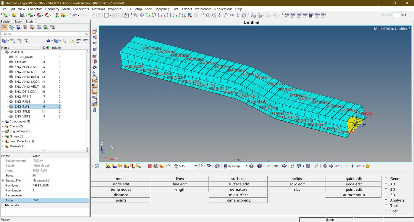
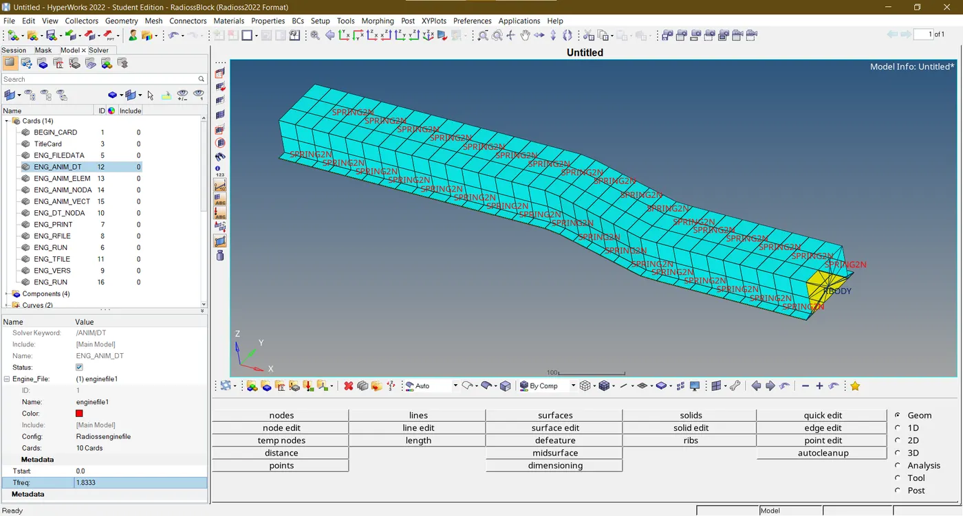
• As per the objective change the number of animation steps during simulation to a minimum of 25 and a maximum of 60. So in the first case, we will keep it as 30 so the frequency time in ENG_ANIM_DT card is computed as follows

T frequency = Termination time/animation time step

= 55 / 30

= 1.8333.

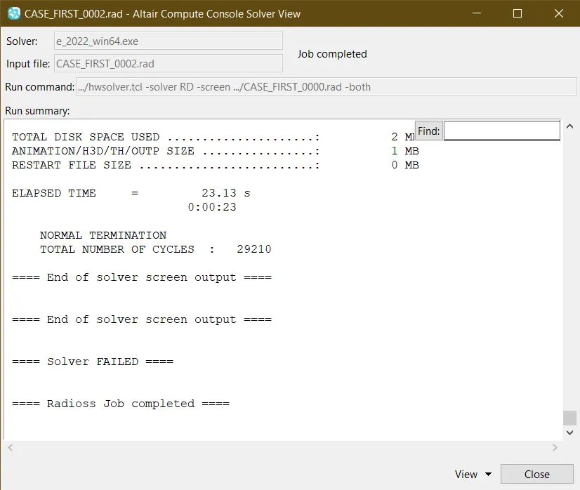
• It failed due to some wrong values in cards and lastly, 45 animation time steps were selected for obtaining T frequency.

T frequency = Termination time / animation time step

=55/45

=1.2

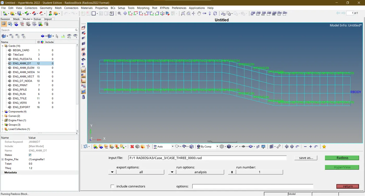
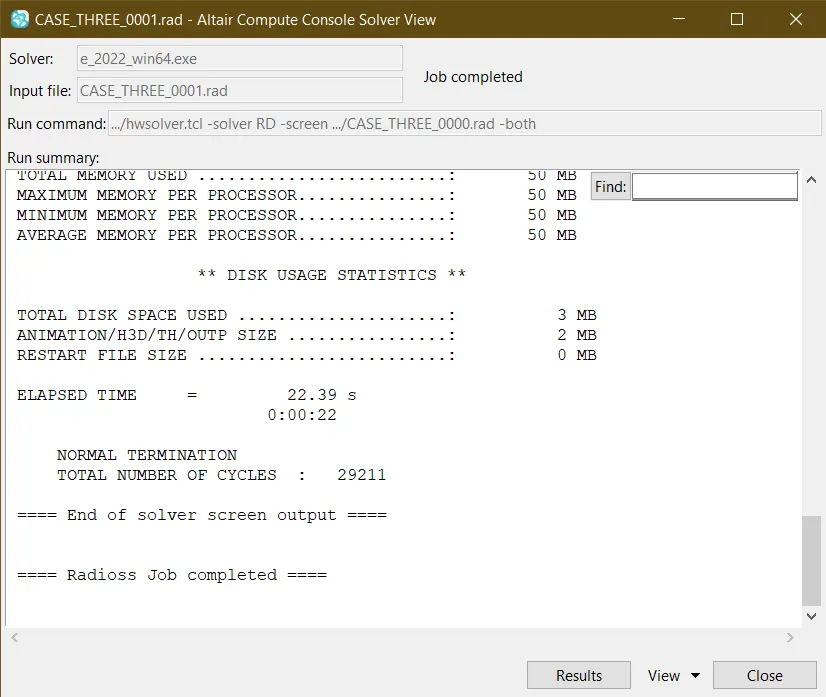
• The RADIOSS job was accomplished and the results were generated for further evaluation.

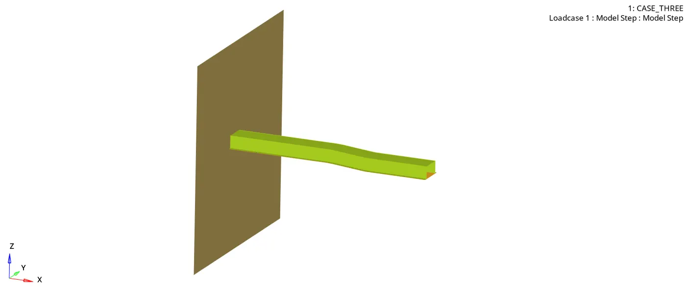
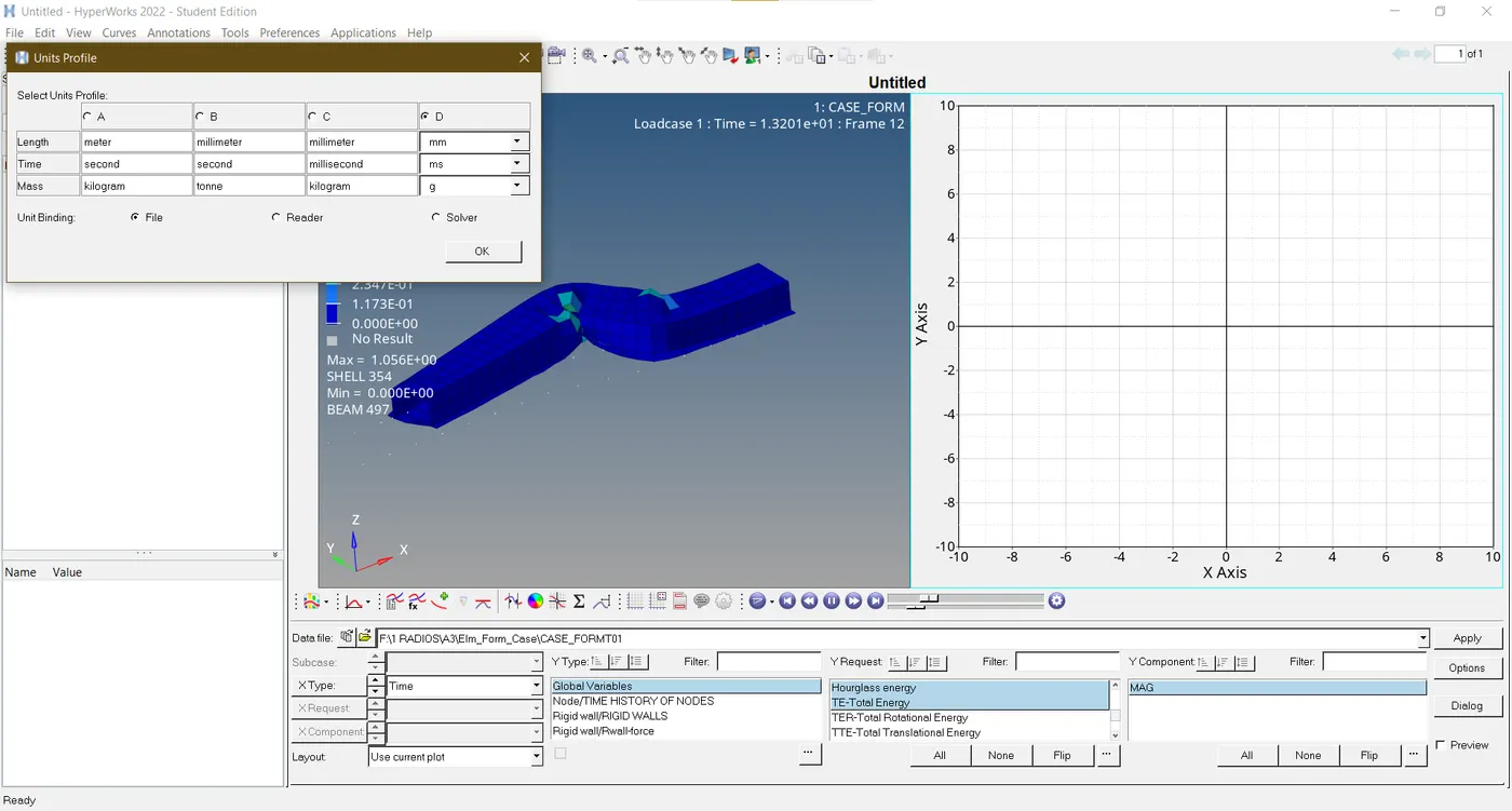
• In Hyperview the simulation was animated by hiding the rigid wall with respective parameters in one window. In another window hypergraph 2D was used to achieve graphs for energies and rigid wall forces using the appropriate unit system selected in the image below.

SHELL FORMULATION SIMULATION

• In this case, the first process is repeated with the addition of shell formulations in Properties cards as prescribed in the Objectives.

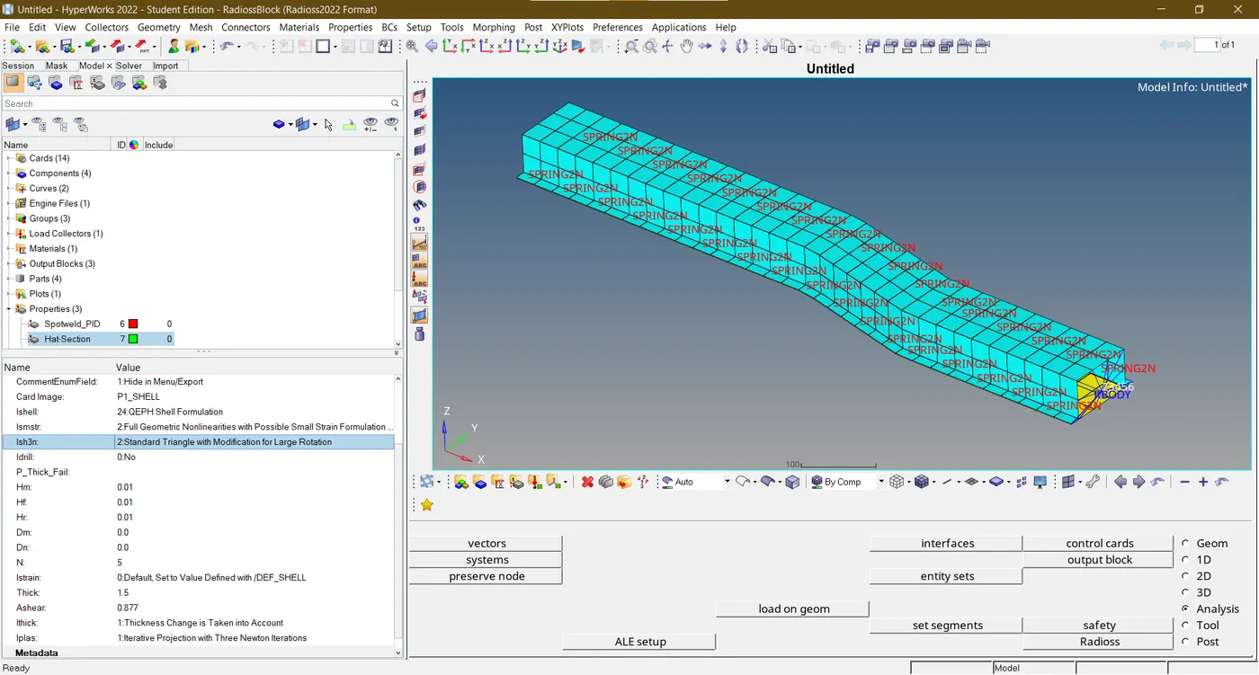
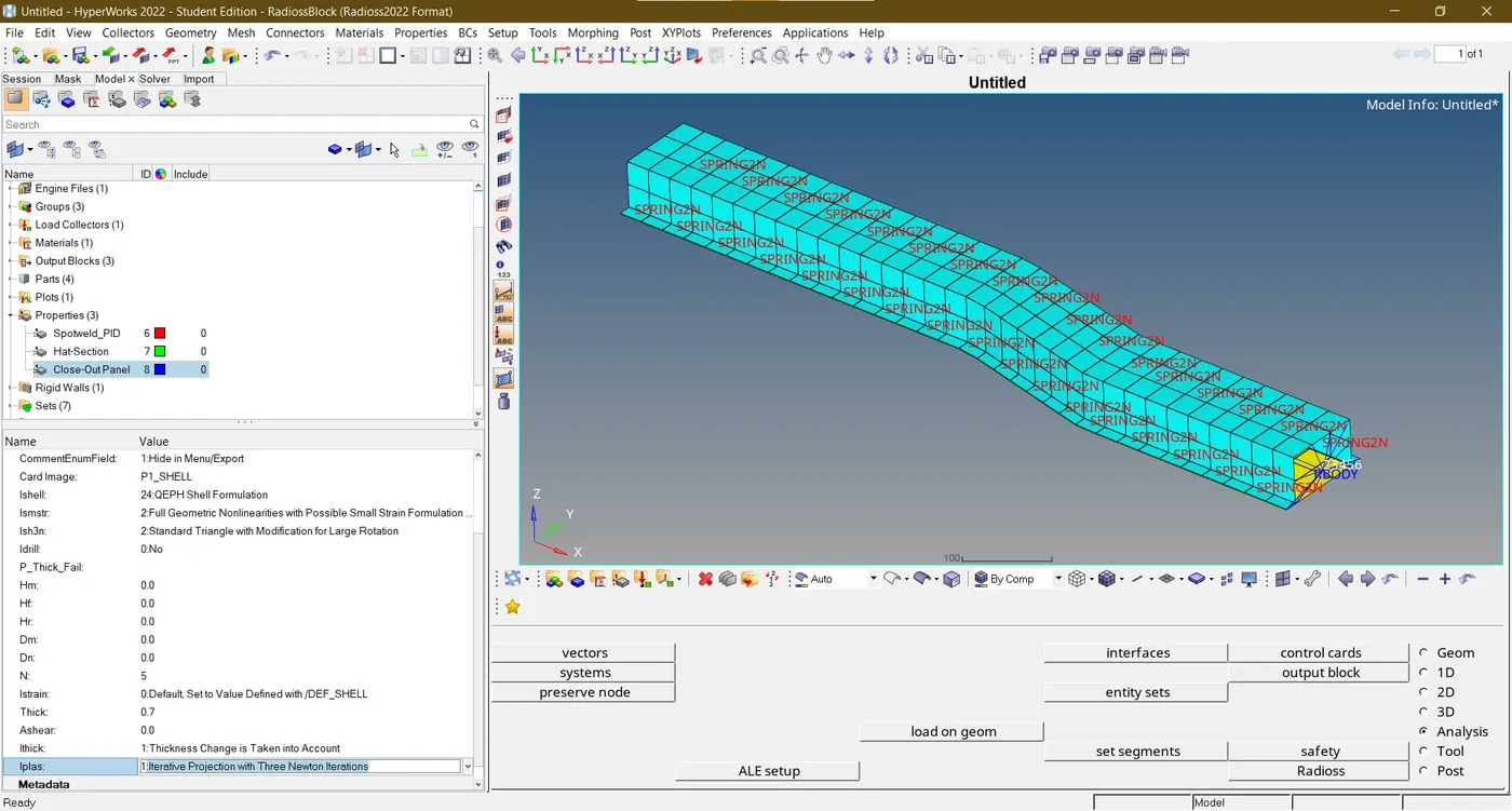
• The solver file is saved under different name in different folder to make a comparison in results further ahead.

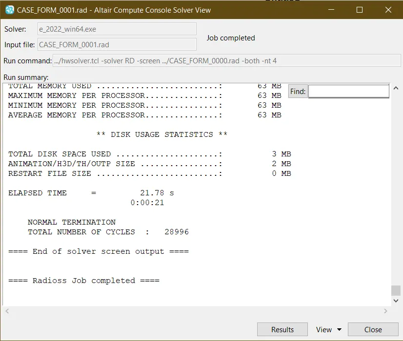
RESULTS

BASE SIMULATION

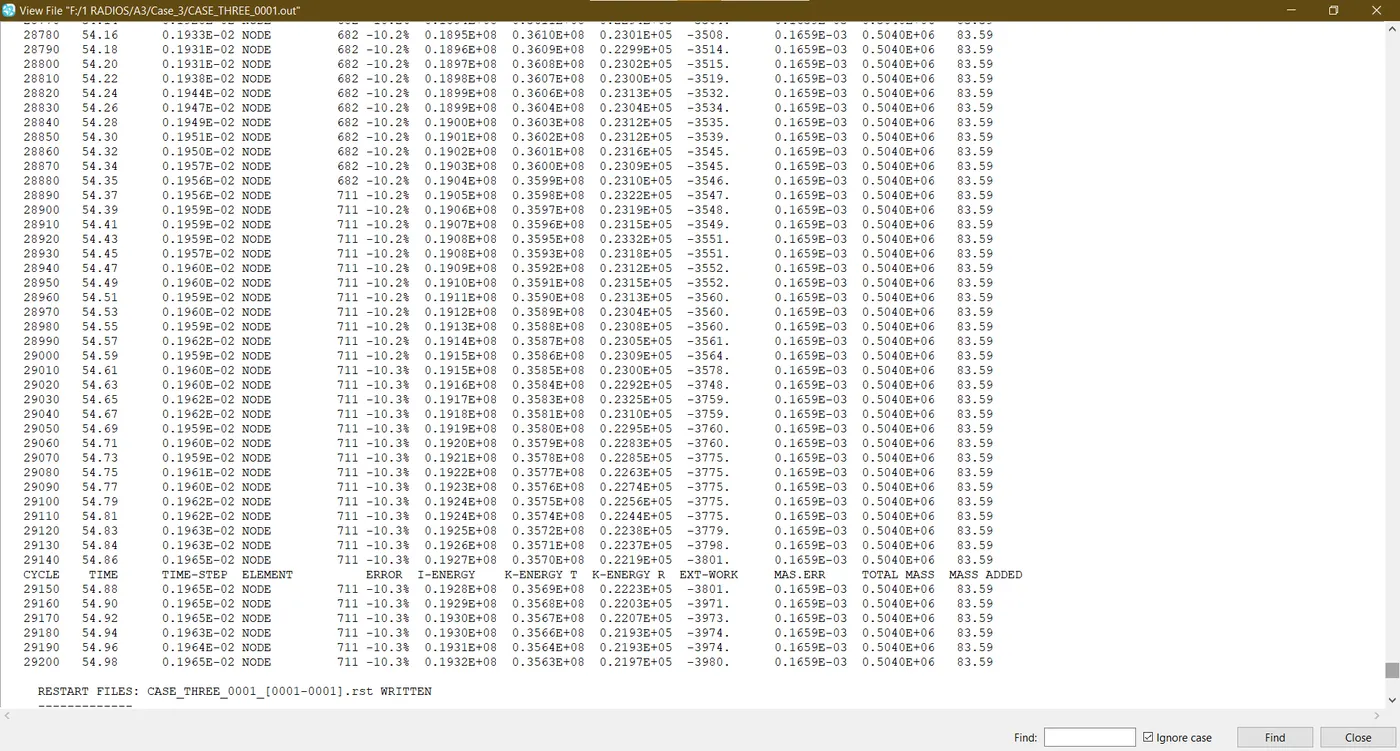
• Better results are taken into consideration within 5%, with an energy inaccuracy percentage of up to 15% allowed. Within a 2% (0.02) threshold, the mass error is accepted.
• In this case, the negative energy percentage means it is releasing and it has a maximum value of 10.2%
• Also, mass error in this case is 0.016% which is way lower than the standard value of 2%

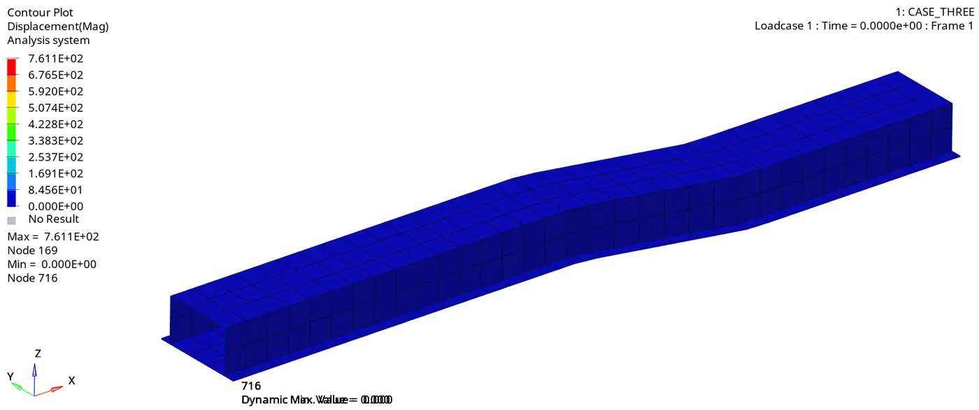
• A maximum displacement of 761 mm is observed in this simulation for this case.

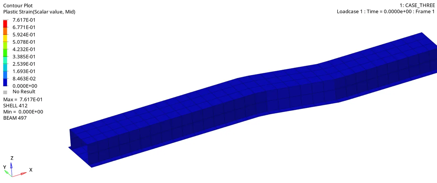
• A maximum Plastic strain of 0.7617 is examined in this simulation for this case

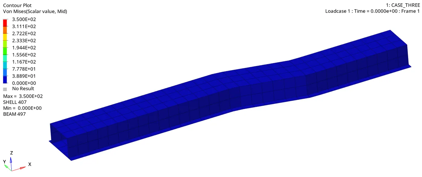
• A maximum Von Mises Stress of 350 MPa is determined in this simulation for this case.

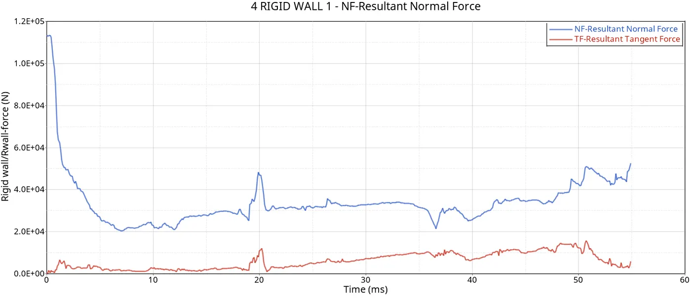
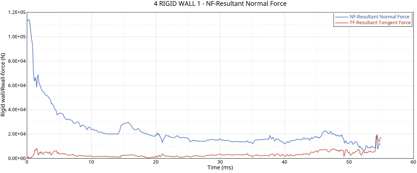
• In Hypergraph 2D the Rigid wall forces are plotted with respect to the termination time. The resultant normal forces designated in this graph are rigid wall forces and the resultant tangent forces are the frictional forces.

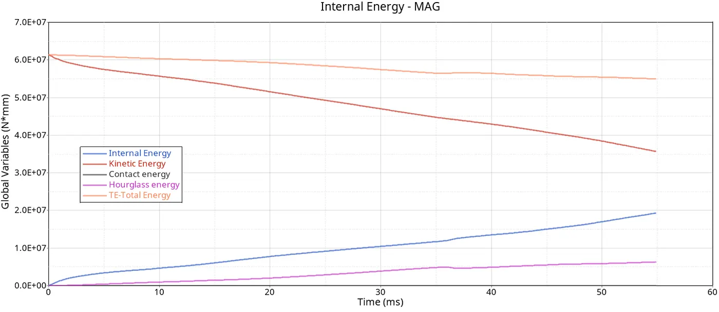
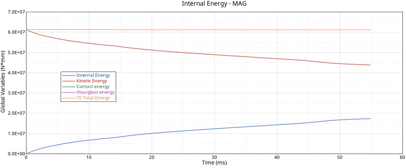
• The energies as displayed below are also plotted with respect to the termination time of the simulation.

SHELL FORMULATION SIMULATION

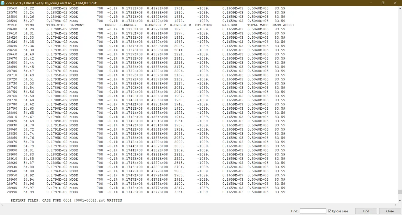
• In this case, the negative energy percentage also means it is released from the system and it has a maximum value of 0.1%
• Also, mass error in this case is 0.016% which is way lower than the standard value of 2%

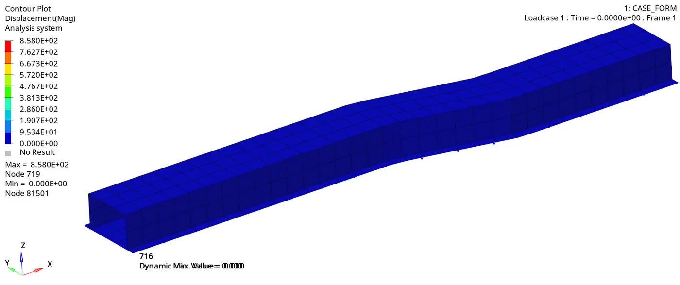
• A maximum displacement of 858 mm is observed in this simulation for this case.

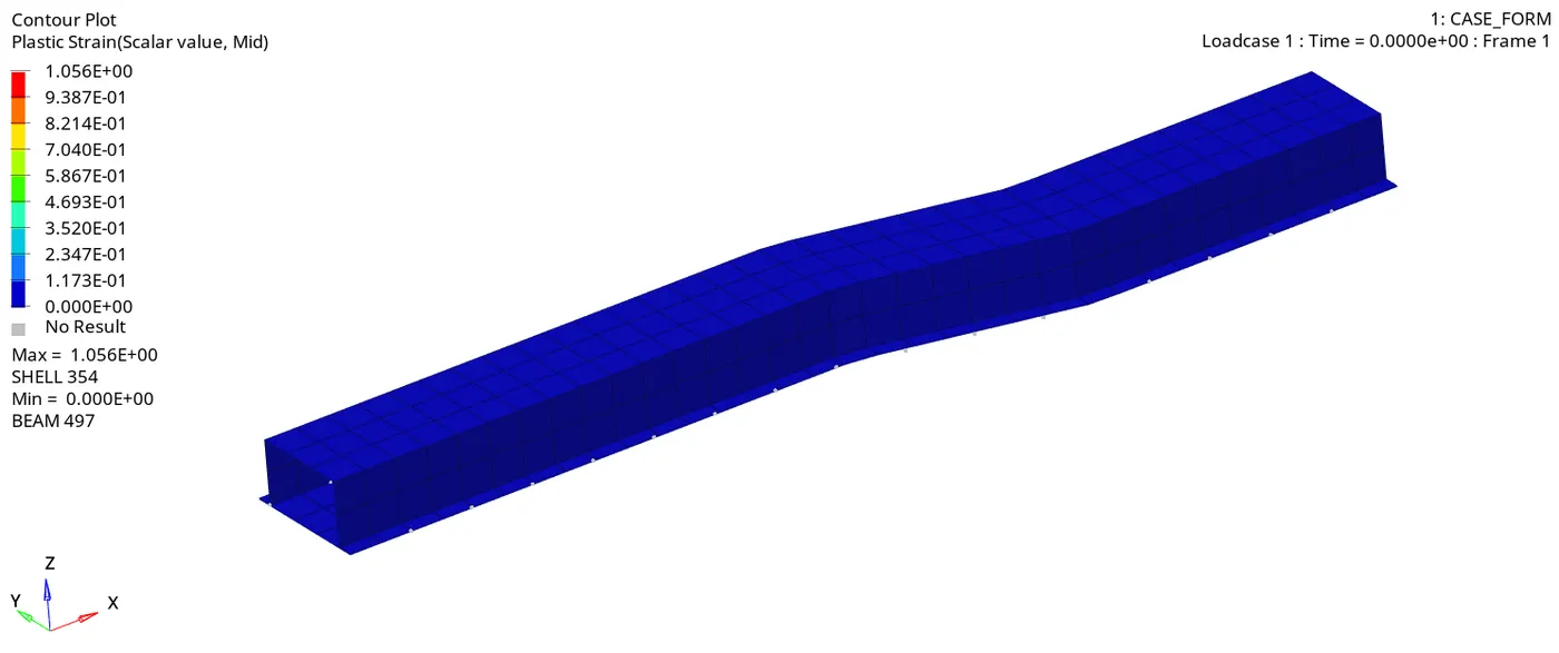
• A maximum Plastic strain of 1.056 is examined in this simulation for this case

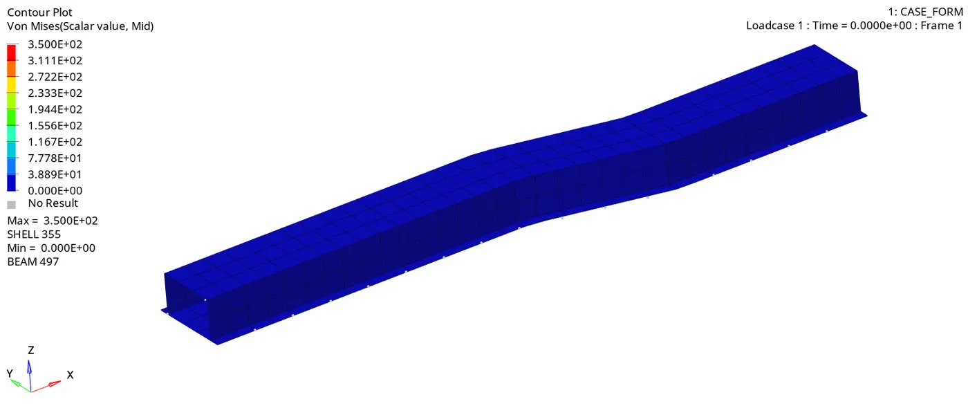
• A maximum Von Mises Stress of 350 MPa is determined in this simulation for this case.

CONCLUSION

1. In the first case, the maximum deformation and plastic strain values are lower than in the shell formulation case.
2. The maximum Von Mises stress assessed in both cases is the same.
3. The mass error percentage in both cases is within acceptable standards. However, the error percentage is reduced to 0.1% in the shell formulation case which is far better than the first case.
4. The rigid wall forces and frictional forces have a huge difference in between throughout the simulation in the first case. In the Shell formulation case, they eventually become equal at the final instant of the end time.
5. The total energy reduces with time in the first case while in the shell formulation case, it remains constant.
6. The Kinetic energy decreases and internal energy increases drastically with a given time in the first case. In the shell formulation case, it decreases and increases slowly contrary to the first case.
7. There is a small quantity of hourglass energy found in the first case while zero hourglass energy is generated in the Shell formulation case.
8. There is zero amount of contact energy found in both cases.
9. Finally, we can claim that the shell formulation case eliminates hourglass energy and reduces the error percentage depending on the respective element properties used. Hence we can achieve efficient and optimum displacements, stresses, strains so forth and so on.