RADIOSS MATERIAL LAWS

INTRODUCTION

The inputs used in any effective simulation are crucial, and to obtain the greatest analysis results, a skilled analyst would always assess and verify the accuracy of the inputs. The type of material selected and the properties offered by the material should be carefully considered. To thoroughly characterize a material for analytical applications, many material attributes could be required as input. Inaccurate results will arise from any ambiguous or nonsensical data submitted during material characterization. When running a simulation, it's critical to select the appropriate materials and supply accurate material data. In the business, RADIOSS has one of the most extensive content and rupture libraries.

The definitions for concrete, foam, rubber, steel, composites, biomaterials, and more all include the material laws and rupture criteria. The desired quality of the model is the primary determinant of the constitutive law selected for a given material. For instance, the constitutive law for standard steel might consider temperature dependence, strain rate, anisotropic hardening, and plasticity. On the other hand, for a regular design, it might only take a basic linear elastic law to provide the required model quality. The analyst made this design decision. In contrast, the program needs to offer a sizable constitutive library to offer models for the materials that are used in real-world applications more frequently. The categorization of most available material laws:

1. Law 1 – Elastic
2. Law 2 – Johnson-Cook
3. Law 25 – Composite
4. Law 27 – Elastic-Plastic Brittle
5. Law 28 – Honeycomb
6. Law 36 – Elastic-Plastic Tabulated
7. Law 42 – Ogden (Hyperelastic)
8. Law 69 – Ogden & Mooney-Rivlin (Hyperelastic)
9. Law 70 – Foam

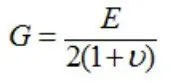
Law 1 – Elastic: /MAT/ELAST uses Hooke's law to define an isotropic, linear elastic material. The linear relationship between stress and strain is represented by this law. It can be used for shell, solid, truss, and beam (type 3 only). Just elastic materials are modelled using this material law. Young's modulus (E) and Poisson's ratio (n) are the only two quantities that determine the stiffness of the material.

It is possible to calculate the shear modulus (G) using n and E:

Only applicable to items with stress levels lower than their yield strength.

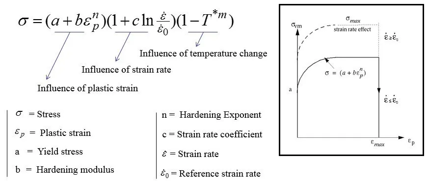
Law 2 – Johnson-Cook: This law uses the Johnson-Cook material model to depict an isotropic elastoplastic material. The material stress is expressed by this model as a function of temperature, strain, and strain rate. There is a built-in failure criterion that is based on the highest plastic strain.

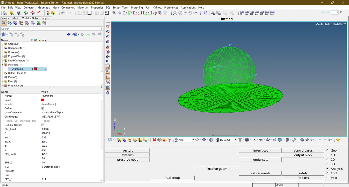
Law 27 – Elastic-Plastic Brittle: This law combines an orthotropic brittle failure model with an isotropic elastoplastic Johnson-Cook material model. Failure is preceded by an accounting for material damage. Damage and failure can only happen under stress. This law solely pertains to shells. The definition of yield surface is the same as Johnson-Cook (Law 2). useful for simulating glass's brittle breakdown.

Four factors are used to describe damage and rupture for each major direction:
et = Strain at the beginning of tensile failure
em = Maximum tensile strain at which the stress in the element is set to a value
dependent on dmax1
dmax = Maximum damage factor

ef = Maximum tensile strain for element deletion

Law 36 – Elastic-Plastic Tabulated: Using user-defined functions for the work-hardening part of the stress-strain curve (e.g., plastic strain vs. stress) at various strain rates, this law simulates an isotropic elastoplastic material.

Note: Plastic strain should have a value of zero at the first point of yield stress functions (plastic strain vs. stress). The default value of ep^max is set to the appropriate value of ep if the last point of the first (static) function equals 0 in stress.

• User-defined function for the work-hardening section of the stress-strain curve
• Available for both brick and shell elements
• Isotropic elastoplastic material
• Elastic region of the stress-strain curve for a material determined by Poisson's ratio and Young modulus
• It is possible to provide material plasticity curves for any number of strain rates.

There are 4 damage and rupture parameters:
• εpmax is the maximum plastic strain for element deletion for any loading (tensile, shear or compression).
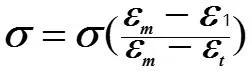
• εt is the beginning of tensile damage. From this point, the stress value defined in the curve is reduced by the factor
where ε1 is the largest principal strain.

• εm is the end of the tensile damage. The stress value is null, but the element is not deleted
• εf is the tensile failure strain value for element deletion

OBJECTIVES

Perform the simulation as per the cases given below.

CASE 1

• Import the FAILURE_JOHNSON_0000.rad file and run the model as it is. Give the title name as Law2_epsmax_failure.

CASE 2

• Import the case 1 rad file, named “Law2_epsmax_failure” and perform the simulation with failure plastic strain (EPS_p_max) and fail_Johson card enabled.

• Changes to be made in /FAIL/JOHNSON card:

• ifail_sh= 1

• Dadv= 1

• Ixfem= 1

• Use the recommended values for the property card.

• Give the title name as Law2_epsmax_crack.

CASE 3

• Import the case 2 rad file, named “Law2_epsmax_crack” and perform the simulation by removing the fail_Johnson failure card. Give the title name as Law2_epsmax_nofail.

CASE 4

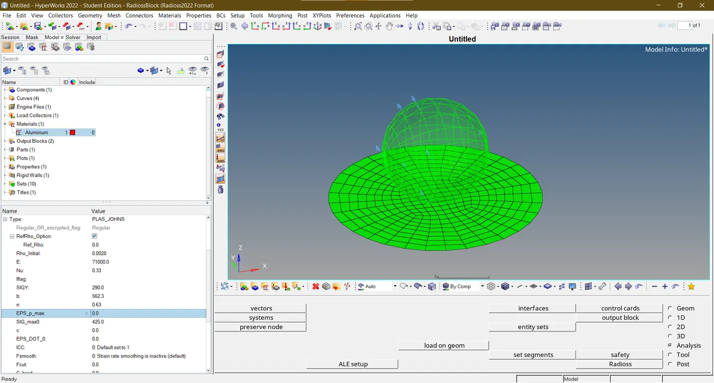
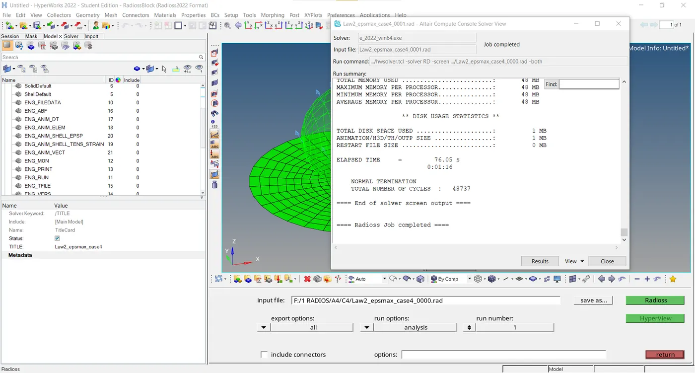
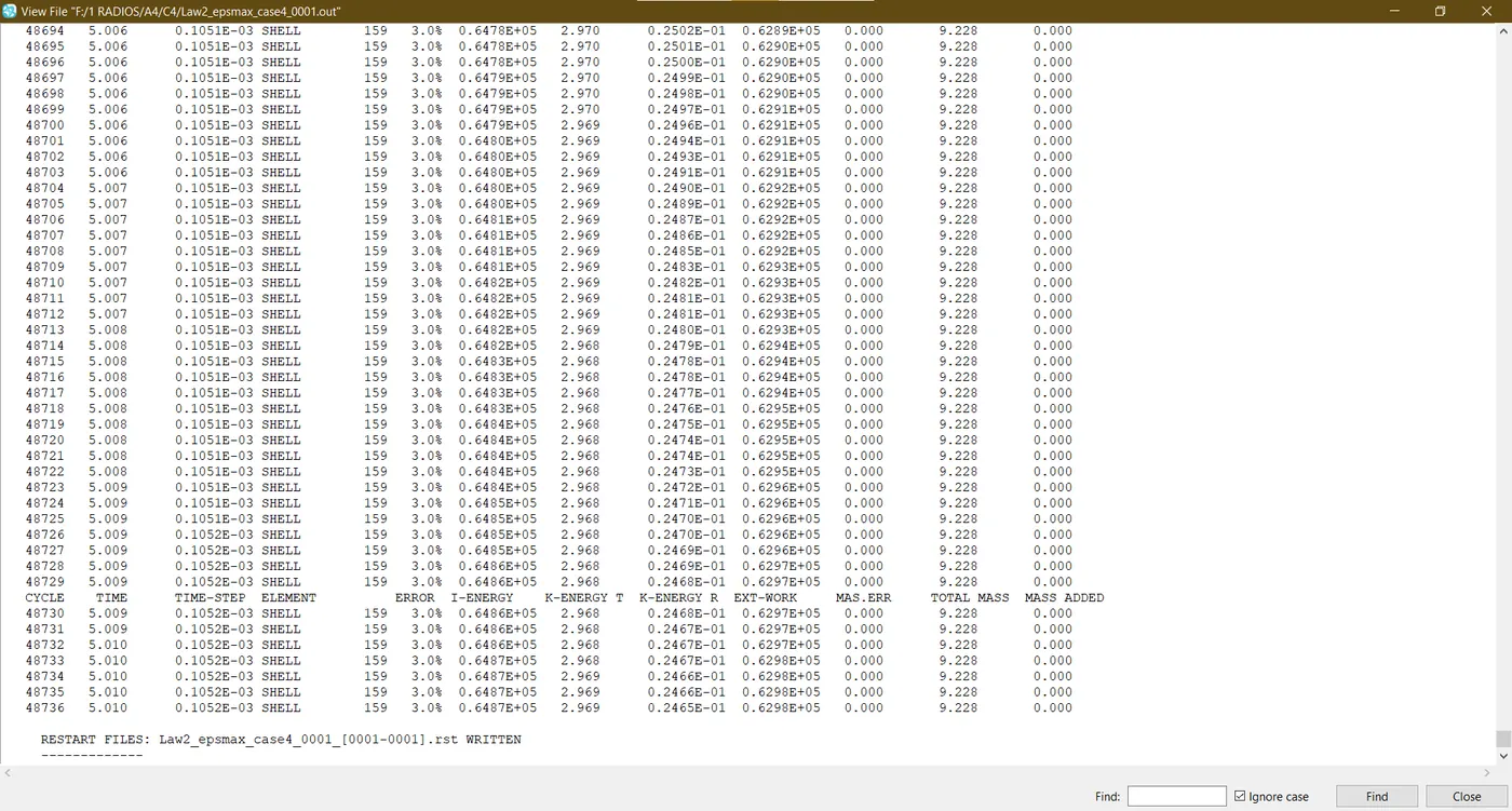
• Import the case 3 rad file, named “Law2_epsmax_nofail” and perform the simulation by removing both the failure plastic strain (EPS_p_max) and the fail_Jhonson failure card.

CASE 5

• Import the case 4 rad file and perform the simulation by changing the material card to Law 1. Keep the same value for rho, E, and nu values.

CASE 6

• Import the case 1 rad file, named “Law2_epsmax_failure” and perform the simulation with the law 36 material card.

CASE 7

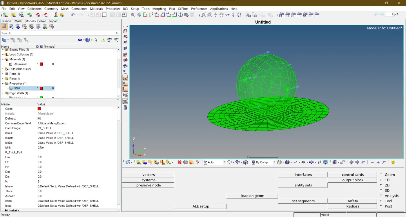
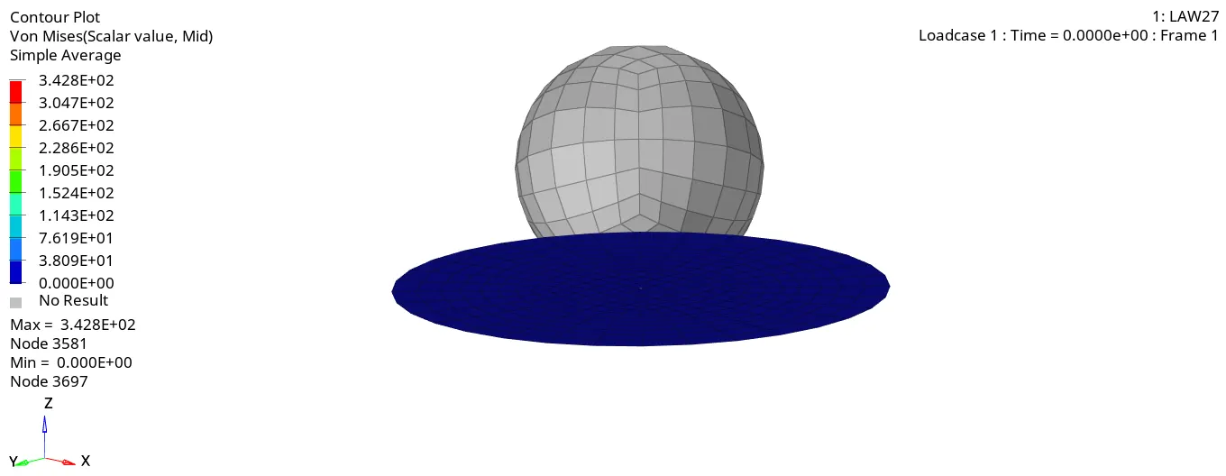
• Open the Law27_0000.rad file and perform the simulation with the Law 27 material card. Use the recommended shell properties.

Compare 7 cases in a tabulated format based on:

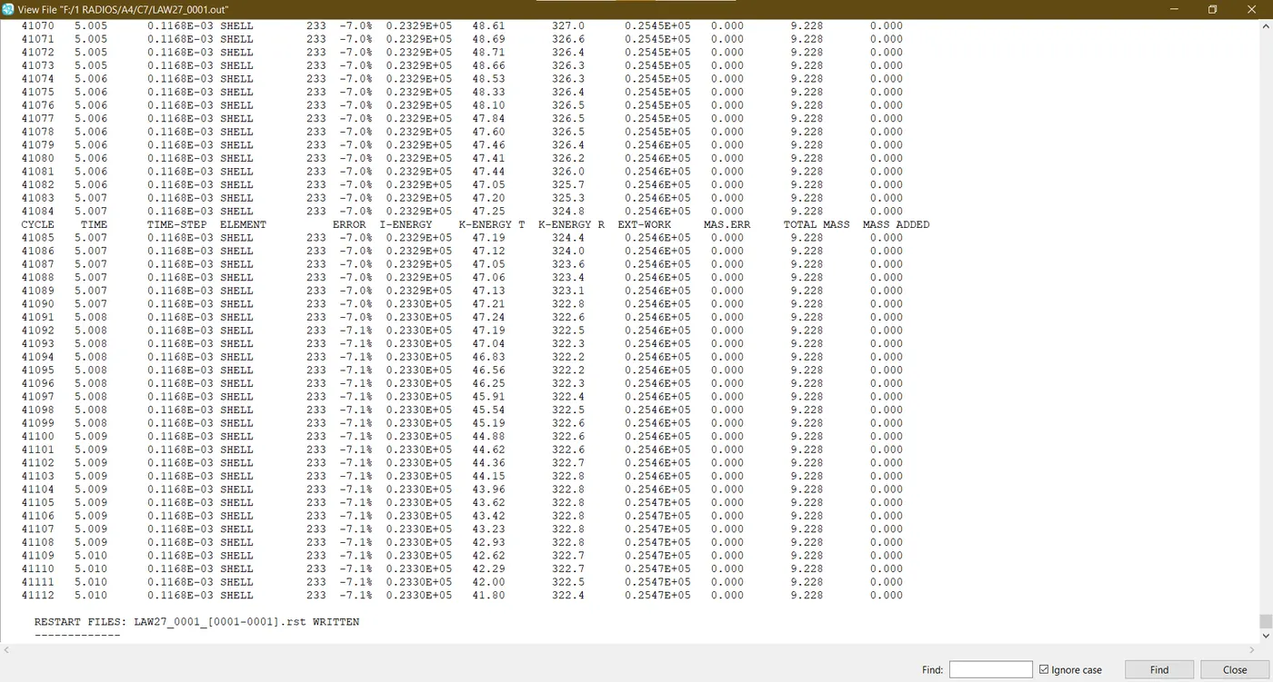
1. The Total number of cycles, Energy error, mass error, and simulation time.
2. Notice the animation of all 5 and describe the animations in brief based on whether the elements are being deleted or cracked.
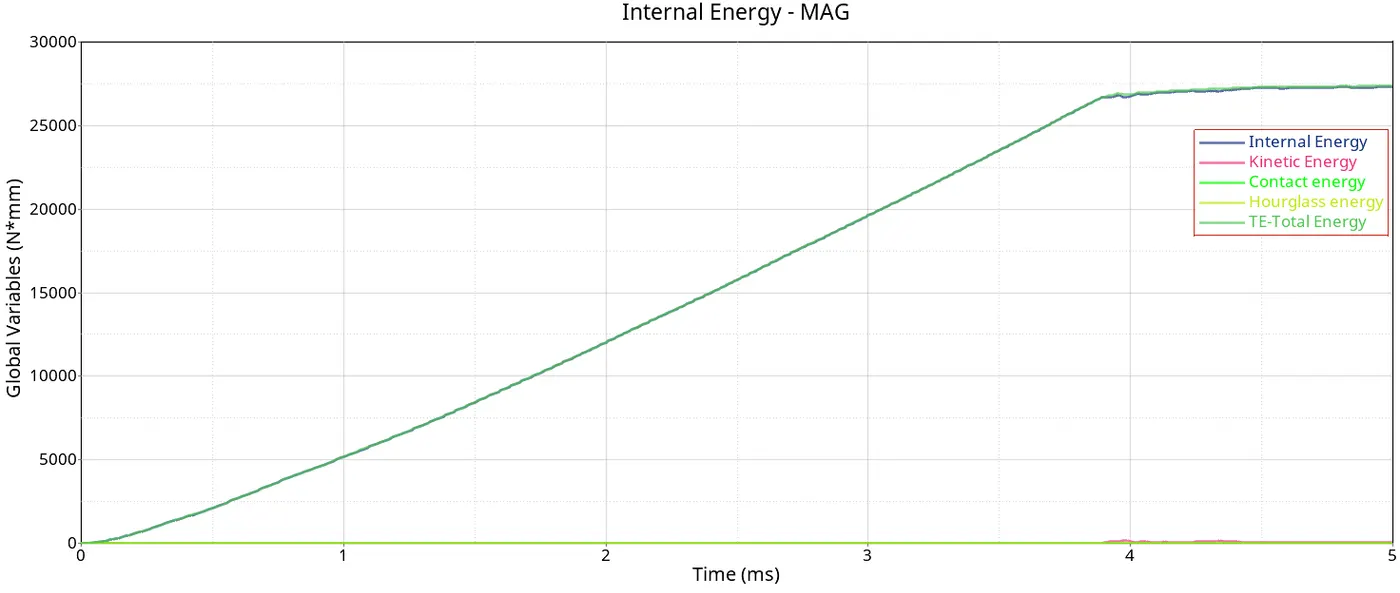
3. Plot energies and notice any difference.
4. Based on all the results, which case would represent the on-field scenario.
5. Prepare a ppt/Docx and list down case-by-case results and your conclusion as to why the failure happened.

PROCEDURE

CASE 1

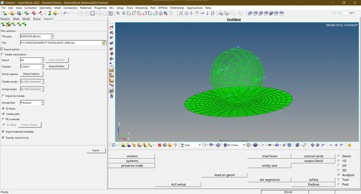
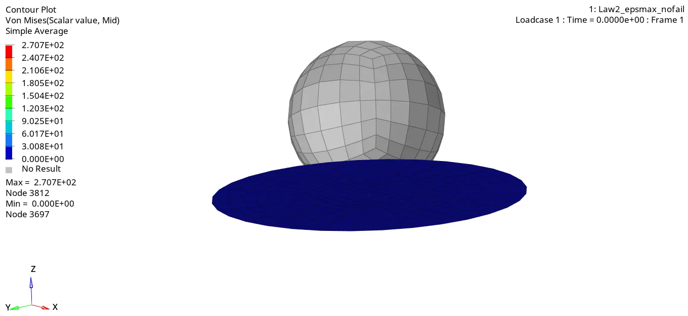
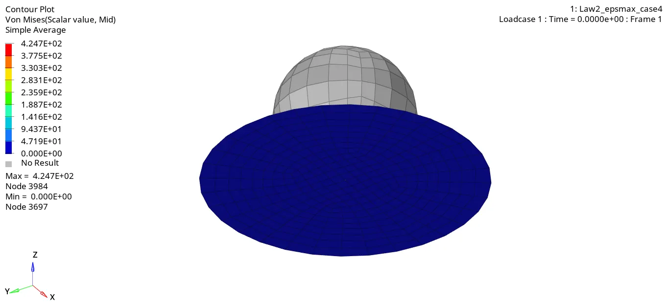
• Import the .rad file given in the assignment in the hyper mesh Radioss solver deck for this case. A circular quad-meshed plate with a rigid ball are clearly visible in the given model for analysis.

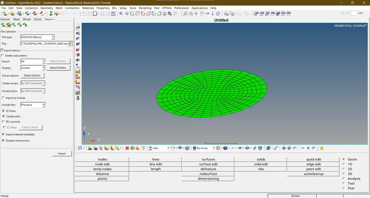
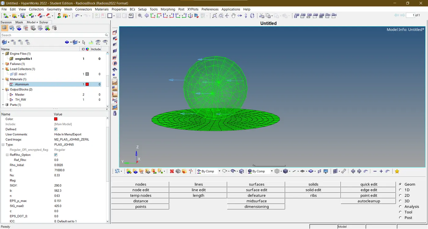
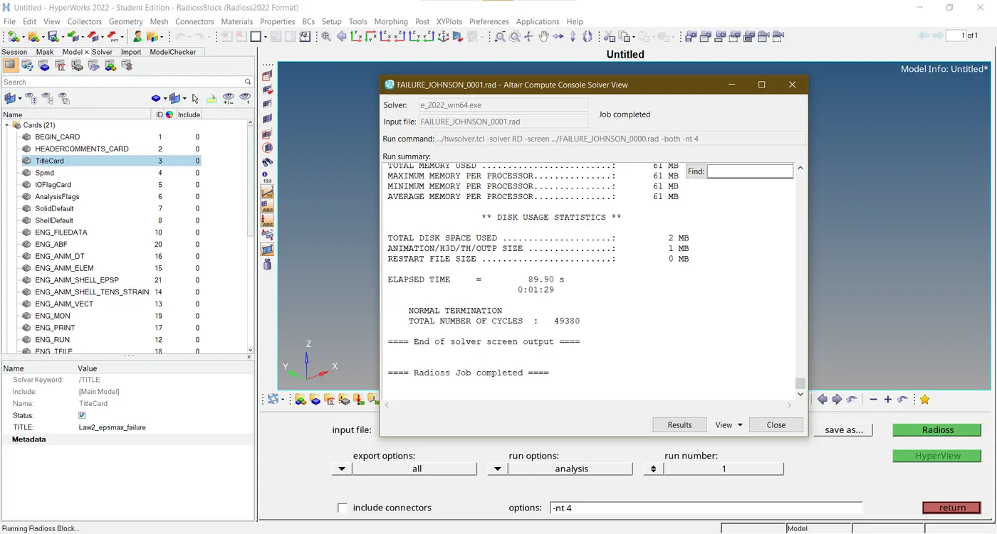
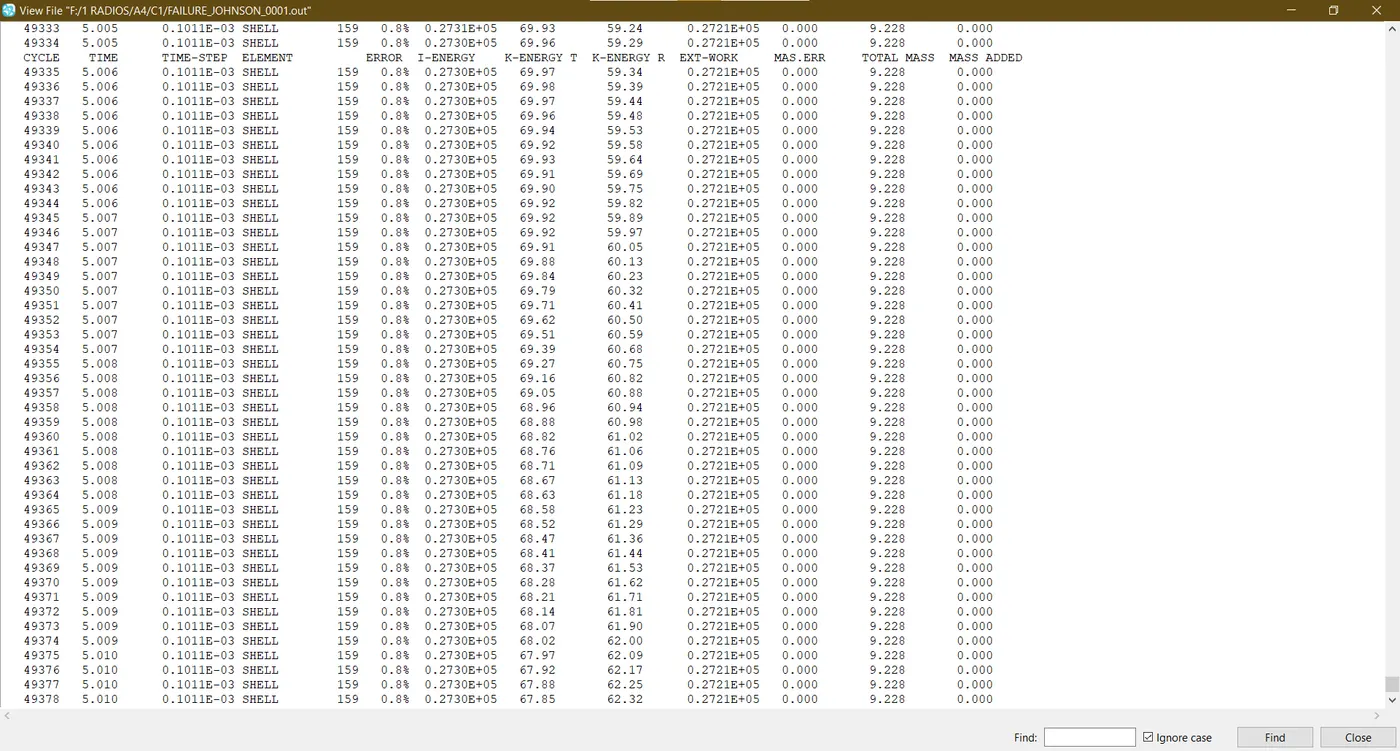
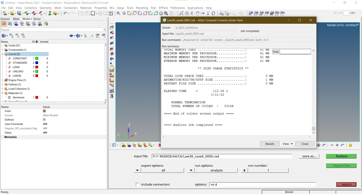
• In this case, no changes are made and the solver is run by saving the file in a different folder named Case 1. Nevertheless, the results and outputs were acquired and tabulated respectively.

CASE 2

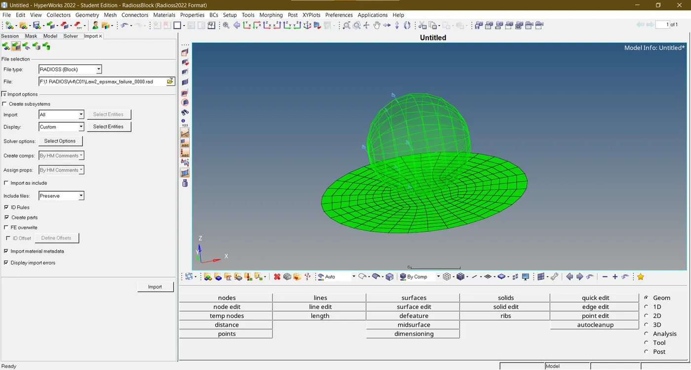
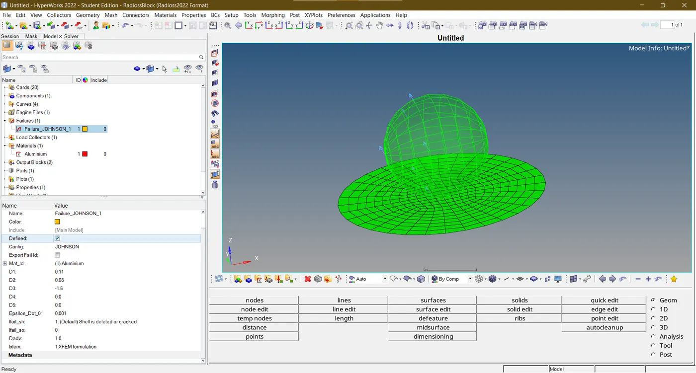
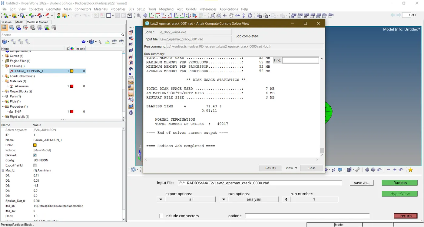
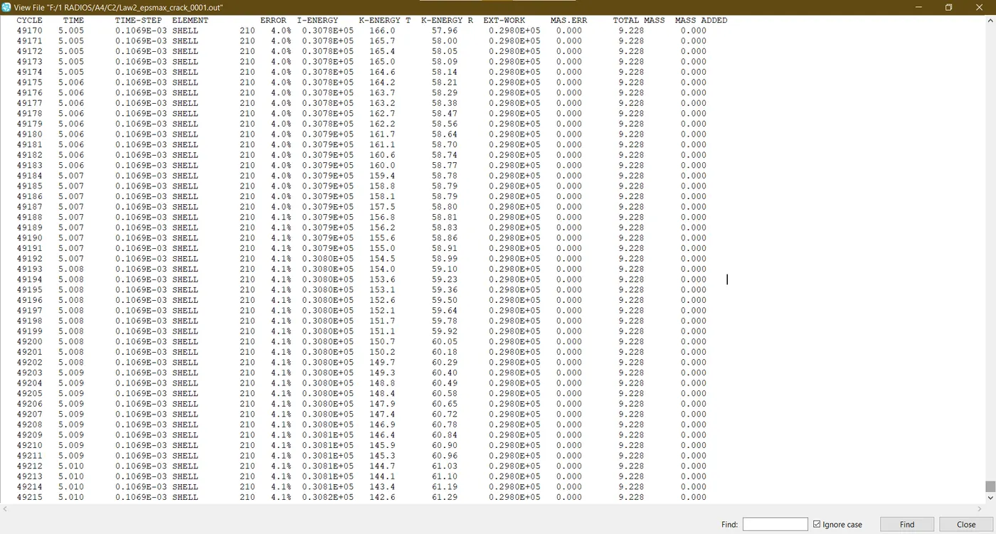
• Initiate the simulation with failure plastic strain (EPS_p_max) and fail_Johson card enabled after importing the case 1 rad file, "Law2_epsmax_failure."

• Changes to be made in /FAIL/JOHNSON card:

1. ifail_sh= 1
2. Dadv= 1
3. Ixfem= 1

• Use the recommended values for the property card.

CASE 3

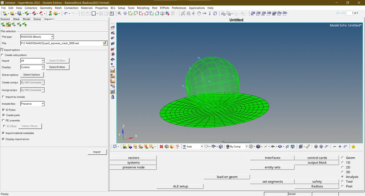
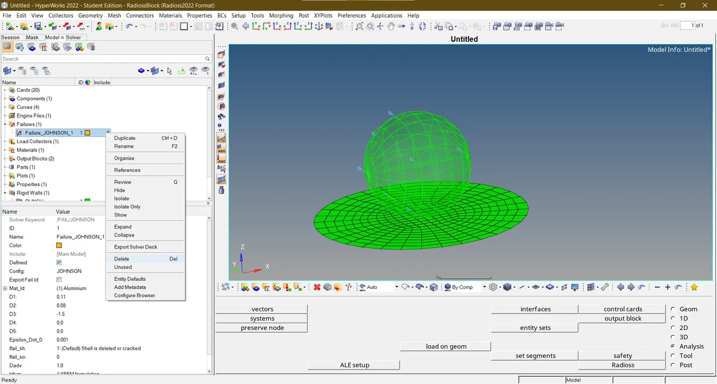
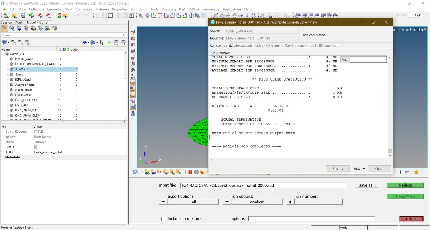
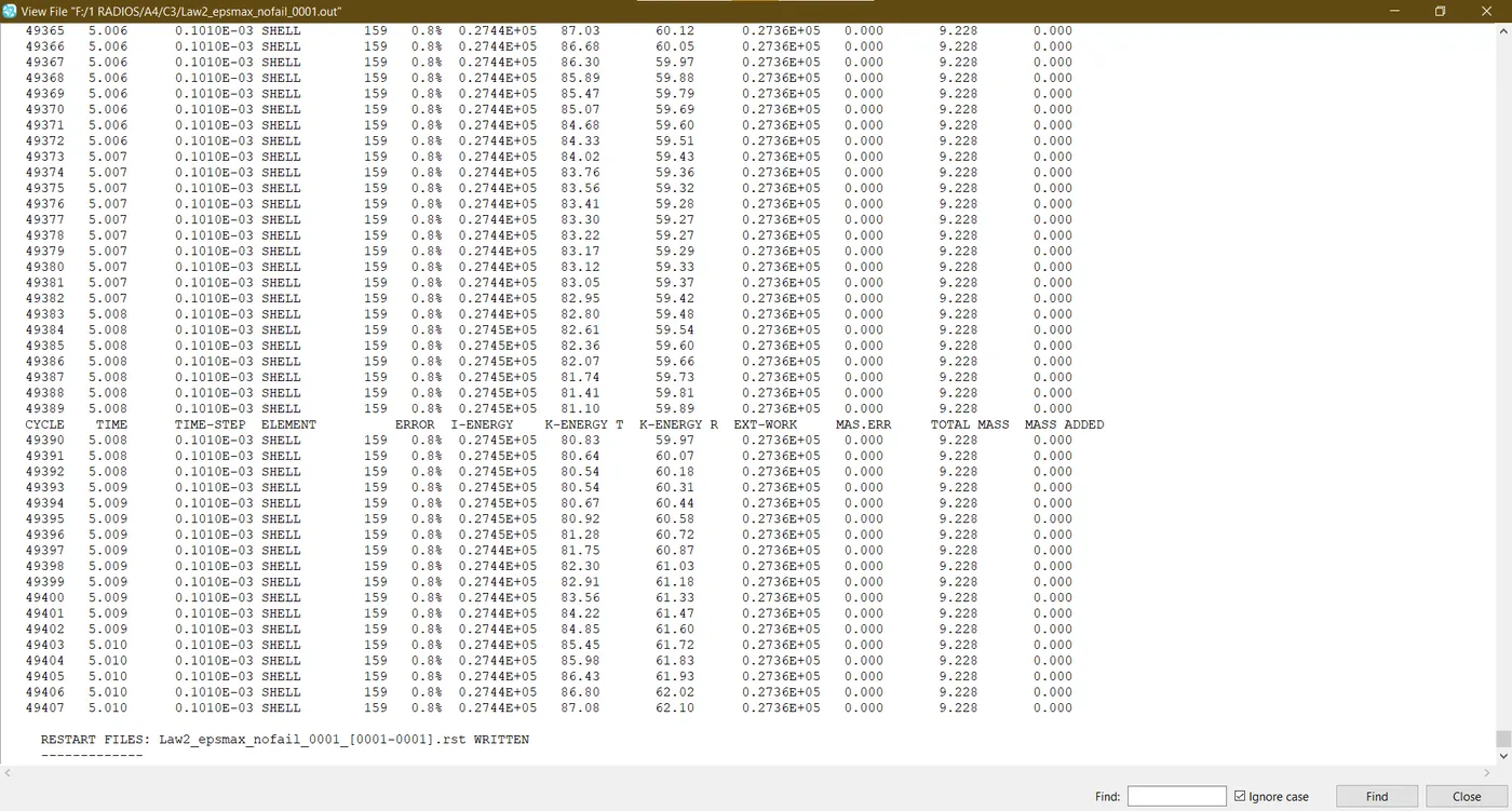
• Remove the fail_Johnson failure card from the simulation by importing the "Law2_epsmax_crack" case 2 rad file. Enter Law2_epsmax_nofail as the title name.

CASE 4

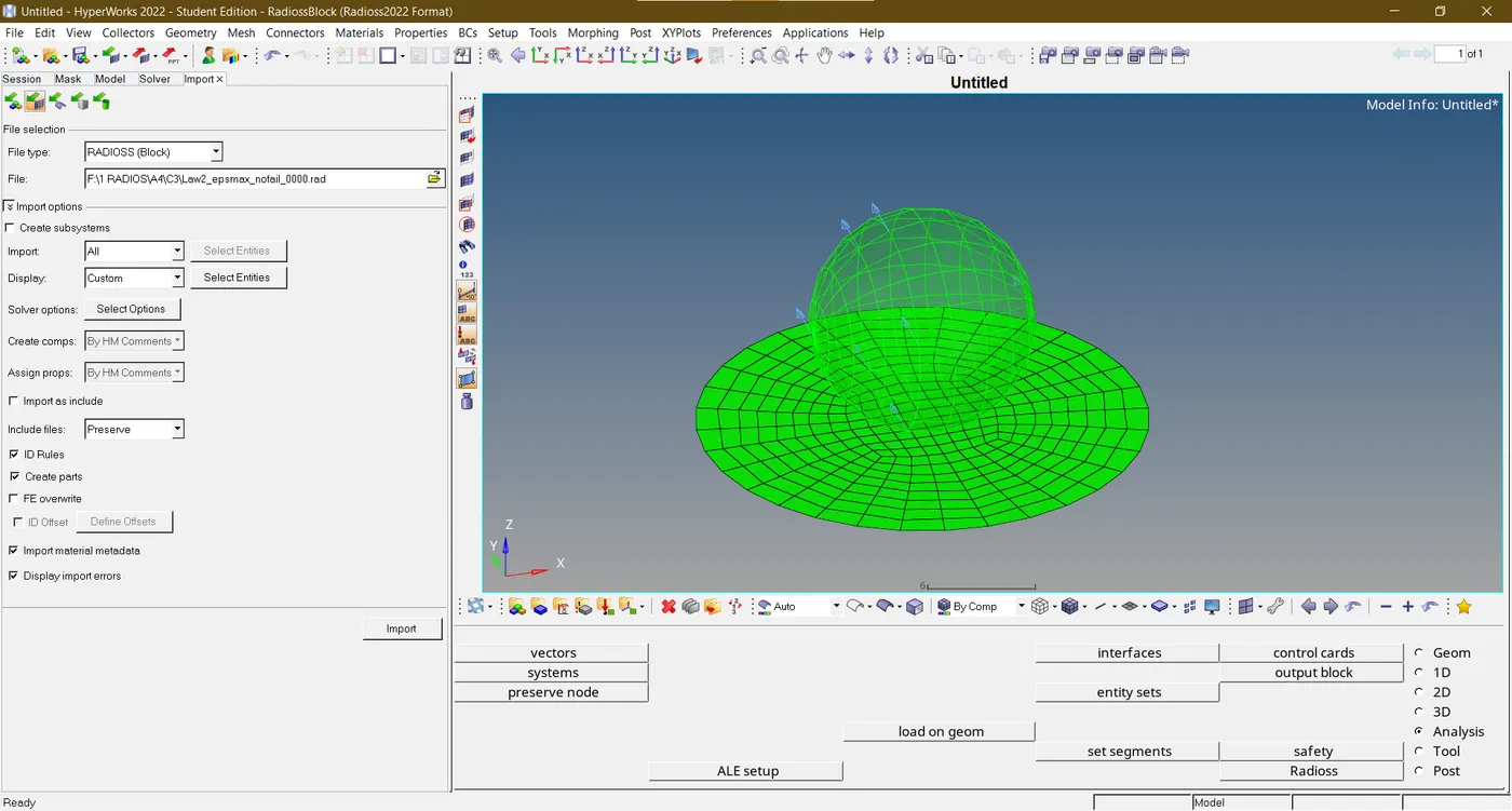
• Import the case 3 rad file, called "Law2_epsmax_nofail," and simulate by eliminating the fail_Jhonson failure card as well as the failure plastic strain (EPS_p_max).

CASE 5

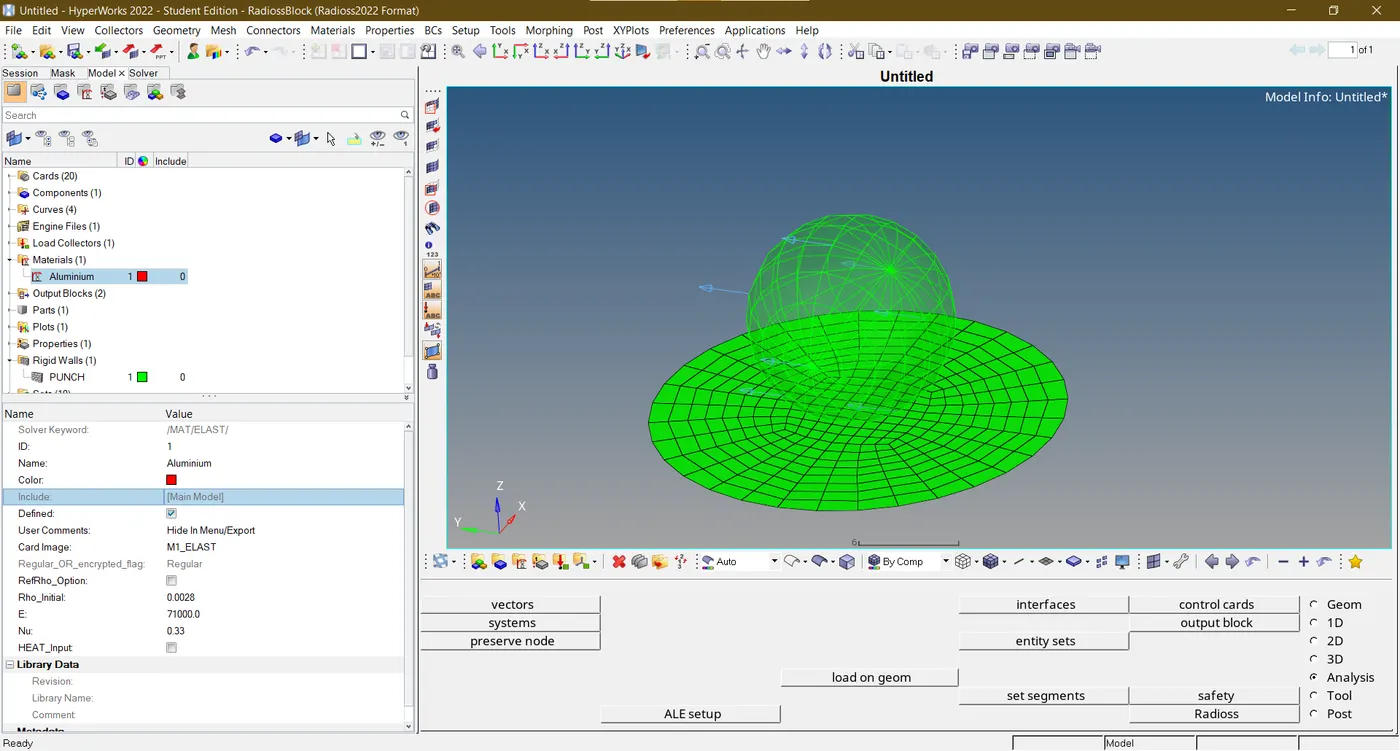
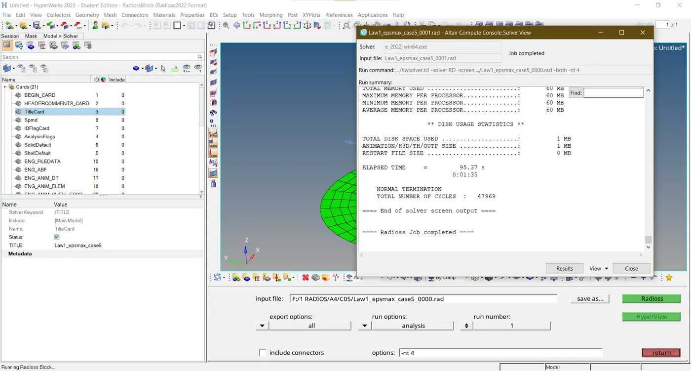
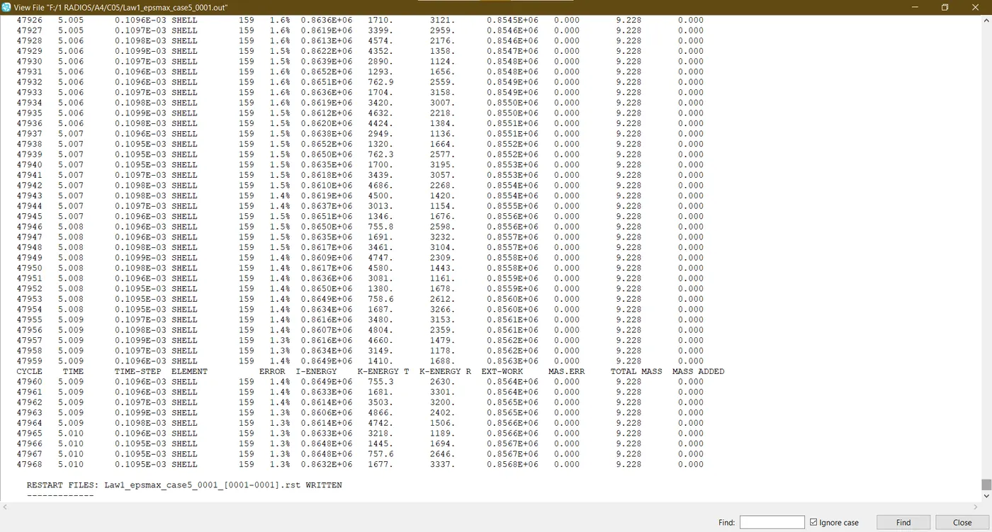
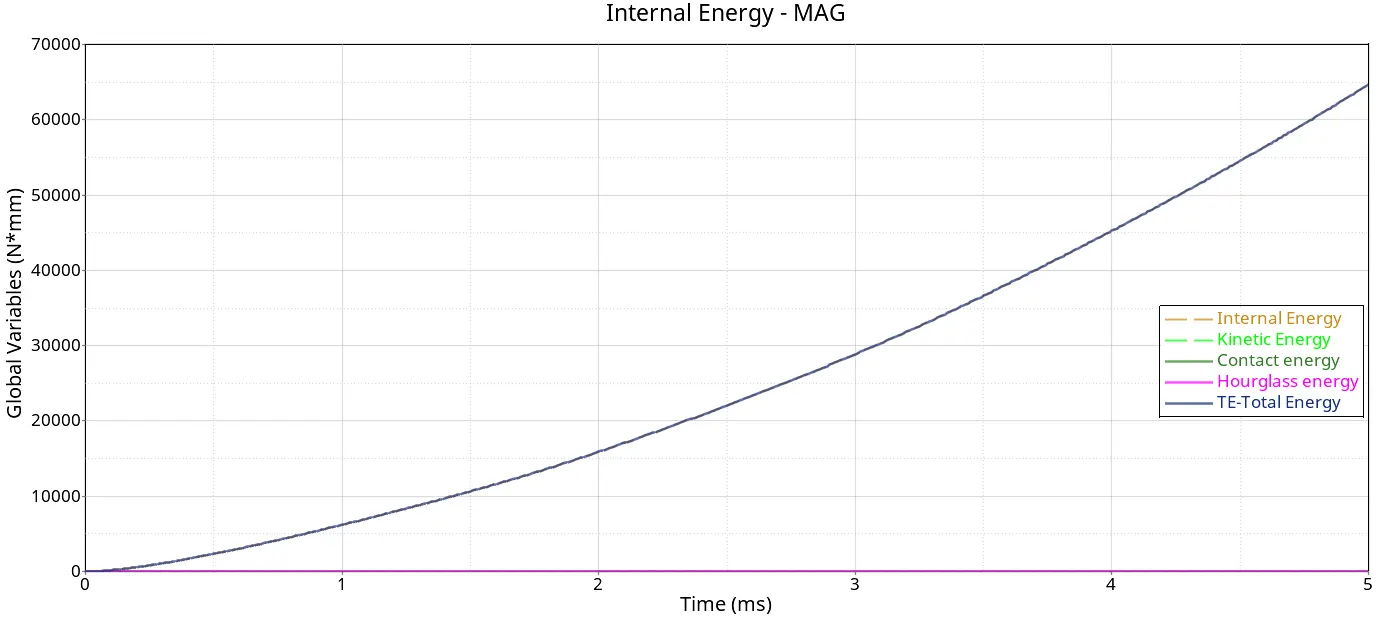
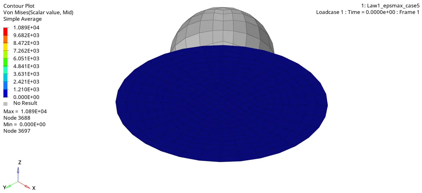
• Change the material card to Law 1 and import the case 4 rad file to start the simulation.

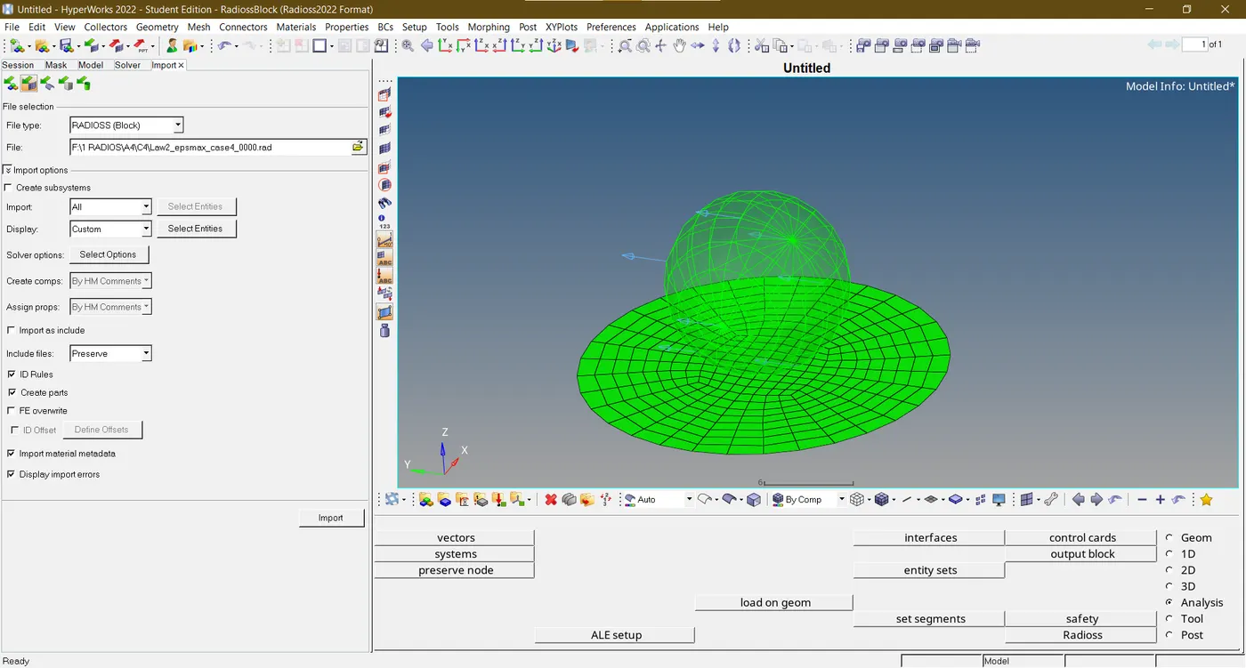
• For the nu, E, and rho values, maintain the same values as used earlier.

CASE 6

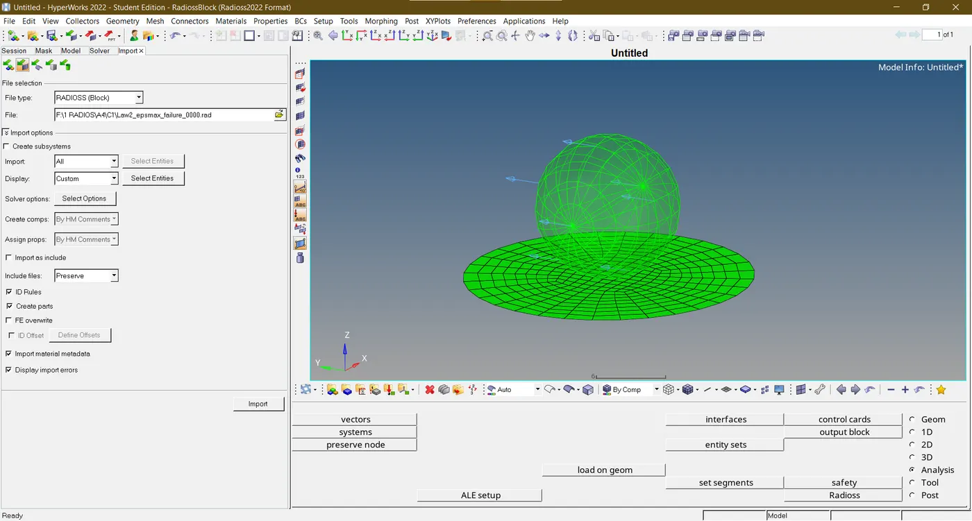
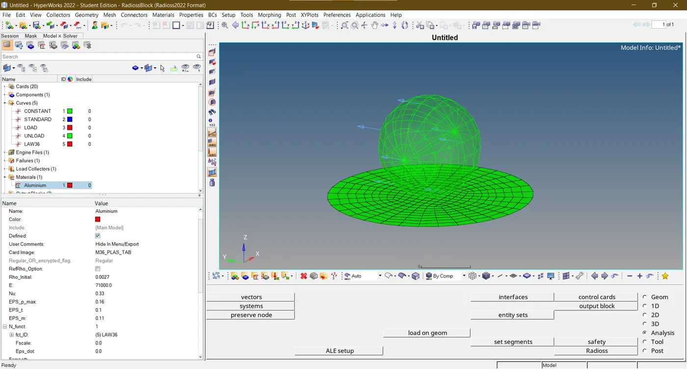
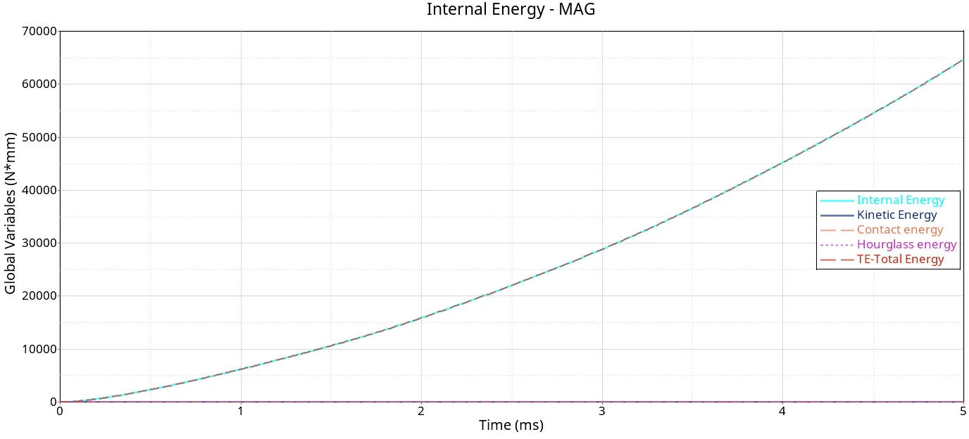
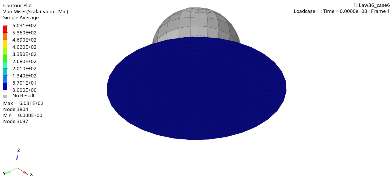
• Utilizing the Law 36 material card, simulate importing the case 1 rad file, "Law2_epsmax_failure."

• Construct a LAW36 curve as prescribed in the assignment and input it into the material card.

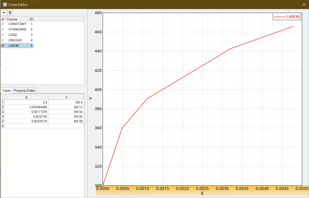
• Use the values of the LAW36 material card as provided in the assignment.

CASE 7

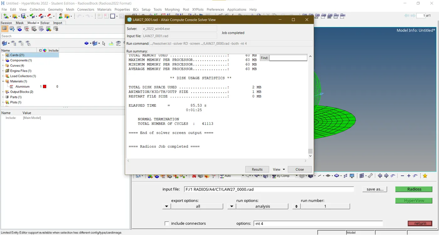
• Utilizing the Law27 material card, simulate by opening the Law27_0000.rad file provided in the assignment.

RESULTS

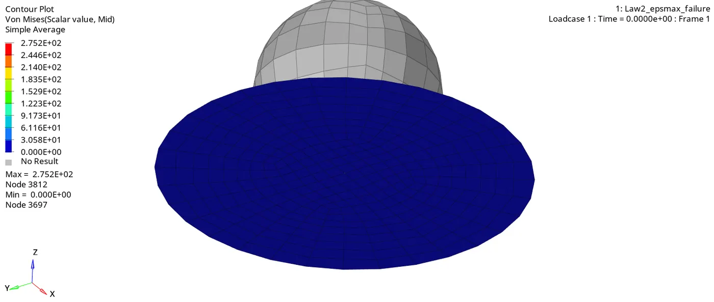
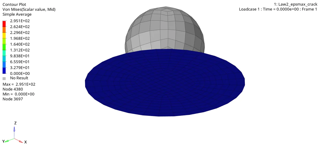
• The post-processing results obtained from Hyperview and Hypergraph 2D of all the cases are displayed as follows:

CASE 1

CASE 2

CASE 3

CASE 4

CASE 5

CASE 6

CASE 7

COMPARISON OF ALL CASES

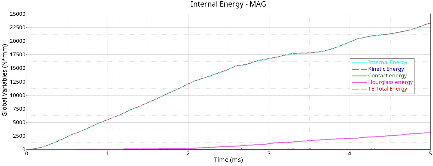
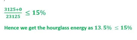
• The hourglass energy is noticed in Case 7 only so the appropriate formula is used

Putting the values from the Energies plot of Case 7 we get the formula as

Simulations	Material LAWS	Total Number of Cycles	Simulation Time (s)	Energy Error (%)	Mass Error	Von-Mises Stress (MPa)	Elements Deleted during the simulation
CASE 1	2	49380	89.9	0.8	0	275	Yes
CASE 2	2	49217	71.43	4.1	0	295	Yes
CASE 3	2	49408	66.37	0.8	0	270	Yes
CASE 4	2	48737	76.05	3	0	424	No, only cracked
CASE 5	1	47969	95.37	1.4	0	10890	No, only cracked
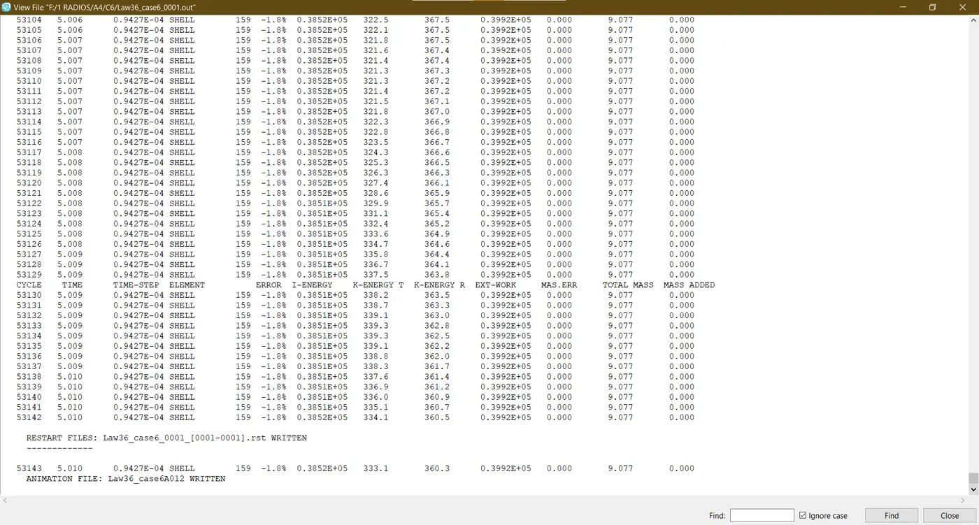
CASE 6	36	53144	112.96	-1.8	0	603	Yes
CASE 7	27	41113	85.53	-7.1	0	343	Yes

• The normal value for contact energy is 0% to 5% of the total energy.
• If the energy error is negative, it means that some energy has been dissipated.
• If the energy error is positive, there is an energy creation.
  
• An energy error of 1% or 2% will be acceptable.
  
• The mass error should be less than 0.05 (5%)

CONCLUSION

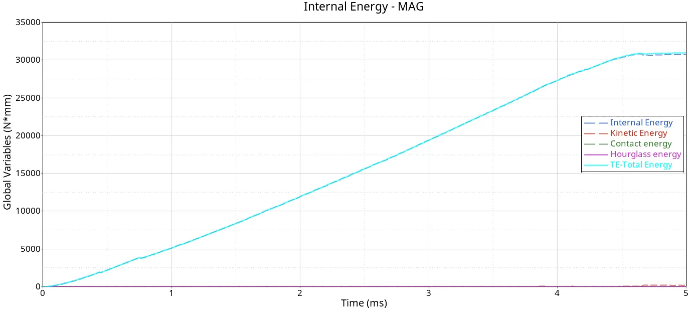
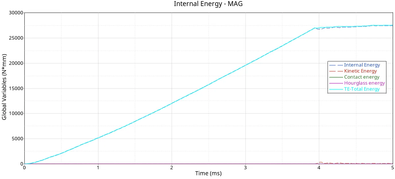
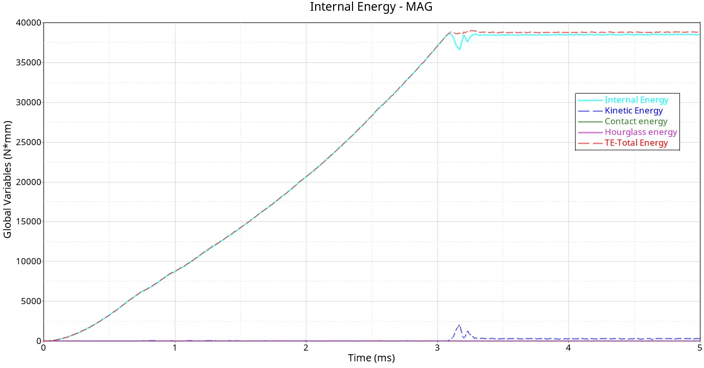
1. The contact energy plotted is 0% in all cases. Except for Case 7 hourglass energy is 0% in all cases.
2. The kinetic energy is 0 for Cases 4 and 5 while for the rest of the cases, it is around 0.5% to 5%.
3. The highest total energy and internal energy is found in Cases 4 and 5. The lowest total energy and internal energy are examined in Case 7.
4. In Cases 1,2,3, and 6 the the total energy increases with a given time until the point of failure and after that, it remains constant.
5. In Cases 4 and 5 the total energy keeps increasing over a given time and forms a curve of hyperbola shape.
6. Case 7 shows an uneven non-uniform increase of total energy over a given simulation time.
7. The total energy and internal energy observed in all the cases are correspondingly equal with the given end time.

• In all these cases Case 3 seems a perfect and suitable example with maximum parameters within a specific threshold of on-field scenario.