Week - 8 Mass Scaling

MASS SCALING

INTRODUCTION:

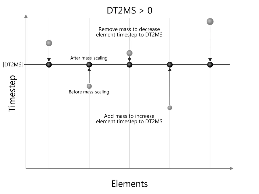
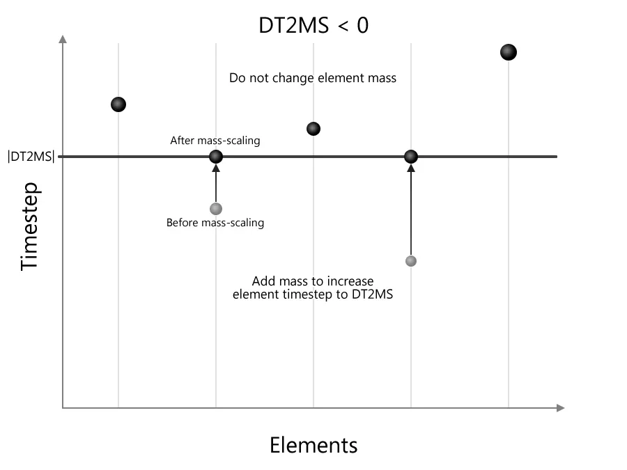
• Mass-scaling refers to the process of scaling an element's mass in explicit simulations in order to modify its timestep. The major goal is to alter (often raise) the global compute timestep, which is constrained by Courant's stability criteria. LS-DYNA supports two methods of mass-scaling when the DT2MS parameter from *CONTROL_TIMESTEP is set to no mass-scaling. When DT2MS is less than zero, LS-DYNA adds mass to each element with a timestep less than abs(DT2MS), so that the element's updated DT equals abs(DT2MS). When DT2MS exceeds zero, LS-DYNA adds mass to elements whose DT is less than abs(DT2MS) and "removes" mass from elements whose DT exceeds zero. DT2MS>0 is rarely used, although DTM2<0 is routinely used to exceed the shortest computed timestep. When using DT2MS<0, care must be taken to ensure that the added mass does not impair simulation accuracy. In dynamic simulations, it is usual practice to limit the percentage of added mass to less than 5% (at the part level). Users can optionally specify ENDMASS in *CONTROL_TERMINATION to end a simulation based on a percentage of added mass based on the model's overall mass. When ENDMAS is greater than zero, LS-DYNA stops when the percentage of added mass reaches ENDMAS, and a report of up to 20 nodes (ordered in descending order of added mass due to mass-scaling) is written to both standard output and the D3HSP file. It should be noted that the proportion of added mass is based on the entire mass of the model, which includes the rigid body, stiff walls, and so on, and may be misleading when viewed on a global scale. LS-DYNA produces the percentage of increased mass at the component level, which is a more accurate indicator of the amount of added mass owing to mass scaling. The concept of mass-scaling is graphically represented below for both DT2MS alternatives.

AIM:

1. The objective is to take the attached model and do the trial and error for mass scaling.
2. Once the mass scaling objective is reached, a histogram should be plotted to compare the runtime with mass scaling trials.
3. Finally, the same model must be run using the implicit solver with the necessary changes, and the implicit and explicit runtimes must be compared.

EXPLANATION:

EXPLICIT ANALYSIS

TSSFAC(0.9)

• The input keyword file is imported into LS-Prepost and we initiate with mass scaling using an Explicit scheme.

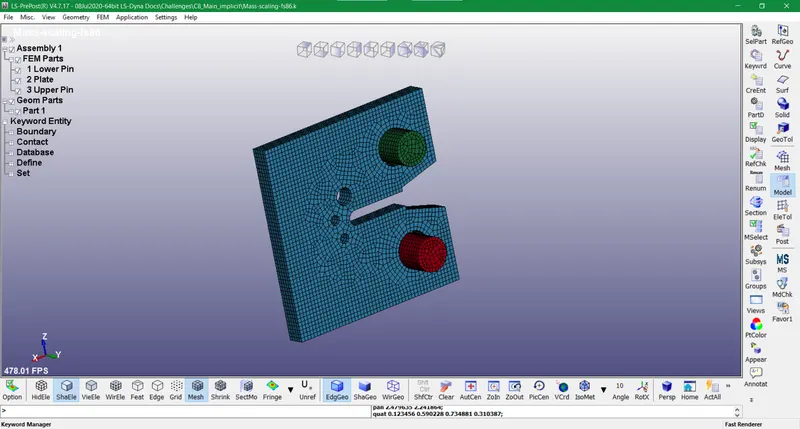
• The simulation is being run with default values in the control time step which is as follows:

1. TSSFAC:0.9 It is the scale factor for the computed time step.
2. DT2MS: -3.500E-05 It is the time step size for mass-scaled solutions.
   

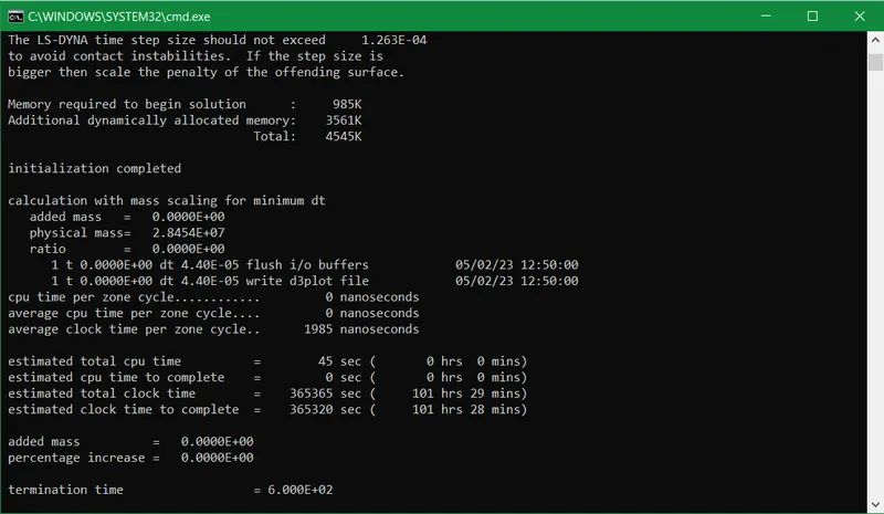
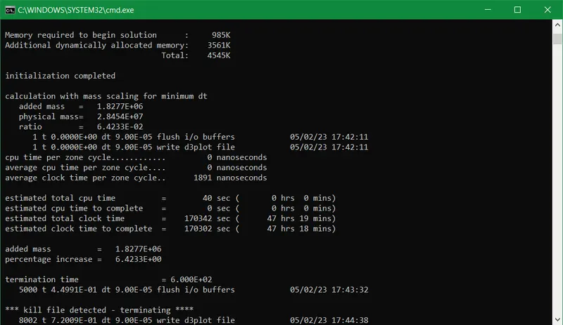
• Henceforth we run the simulation with these default values in the control timestep card in the given input keyword file. There is no percentage increase in mass by the values provided above. So we regulate the DT2MS values by trial and error method and run the simulation several times until we get a percentage increase of mass near around 8%. In this case, we keep TSSFAC as 0.9 for all DT2MS values and will change it in the next case.

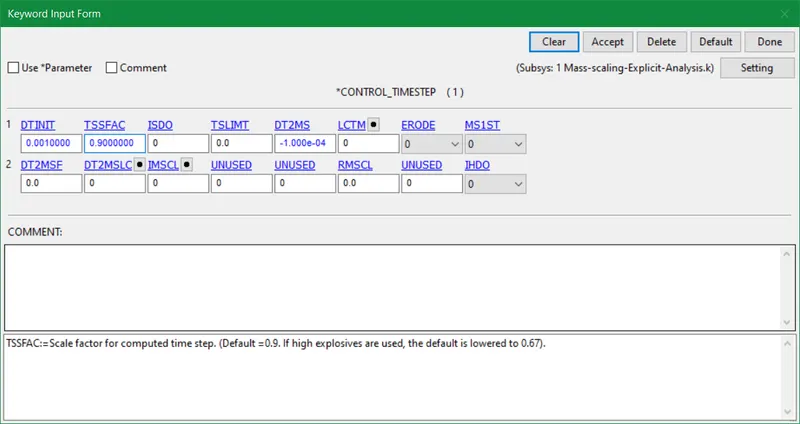
DT2MS -1.000e-04

DT2MS -1.027e-04

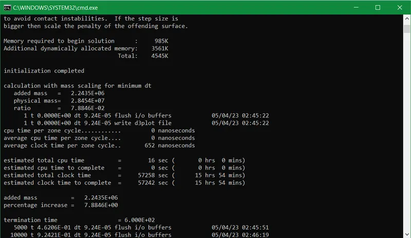
DT2MS -1.028e-04

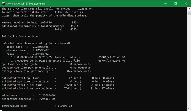
DT2MS -1.029e-04

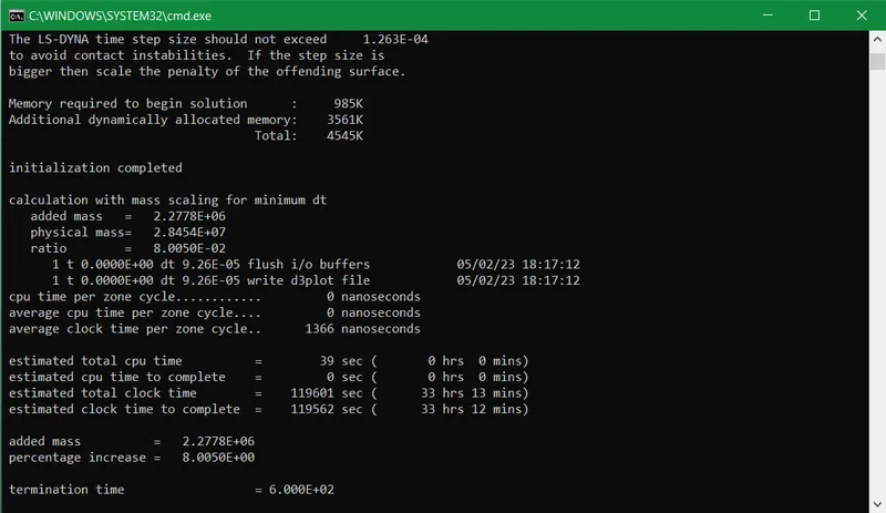
DT2MS -1.030e-04

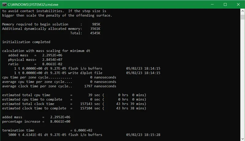
DT2MS -1.031e-04

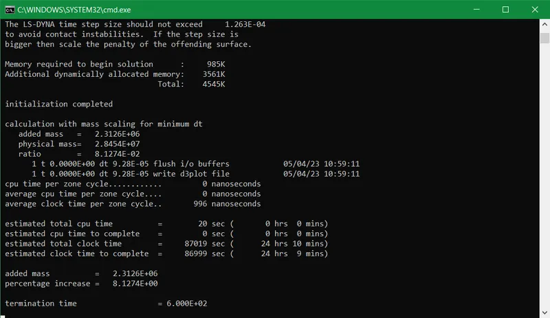
DT2MS -1.032e-04

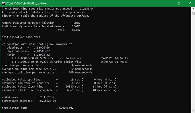
DT2MS -1.100e-04

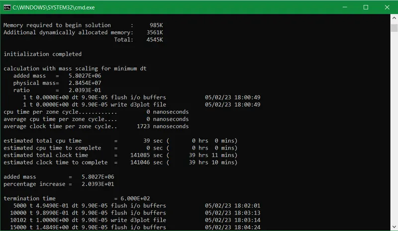
DT2MS -1.500e-04

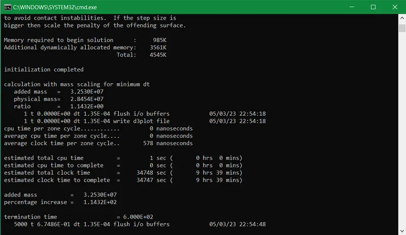
TSSFAC(0.8)

• In the last case, we formulated a sudden change in total clock time with respect to the change in DT2MS values respectively. At -1.029e-04 we achieved approx 8% percent increase in mass for the last case. The same process is followed in this case except the TSSFAC value is inserted as 0.8

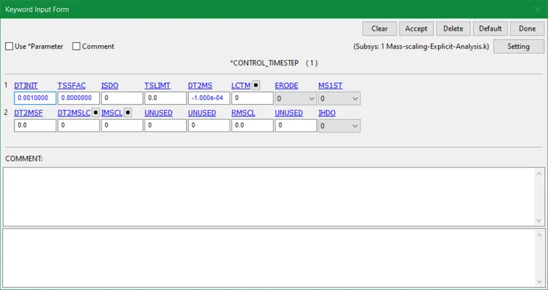
DT2MS -1.000e-04

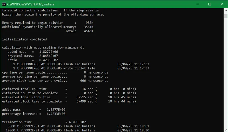
DT2MS -1.027e-04

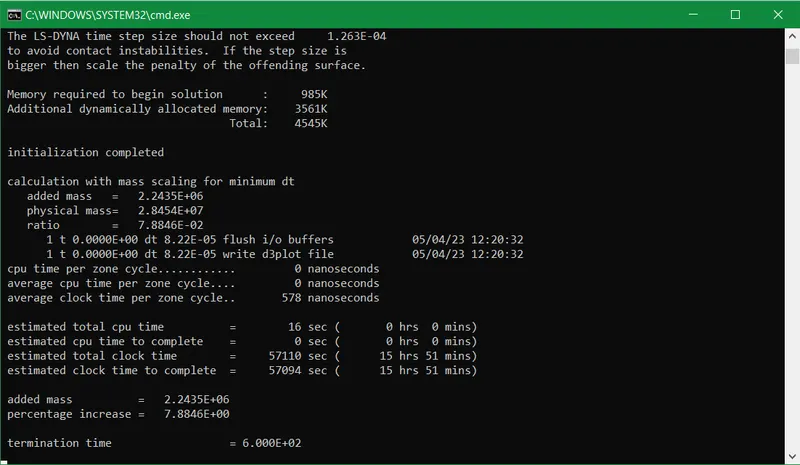
DT2MS -1.028e-04

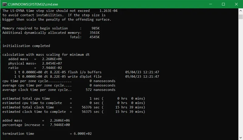
DT2MS -1.029e-04

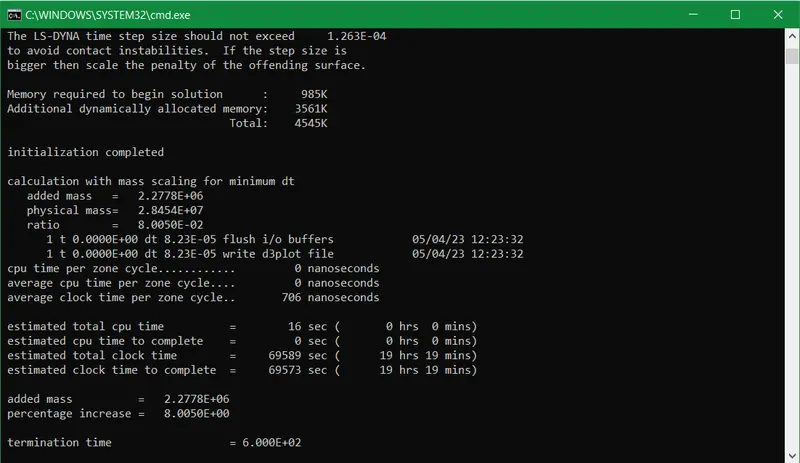
DT2MS -1.030e-04

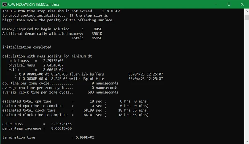
DT2MS -1.031e-04

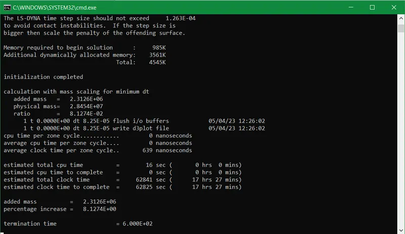
DT2MS -1.032e-04

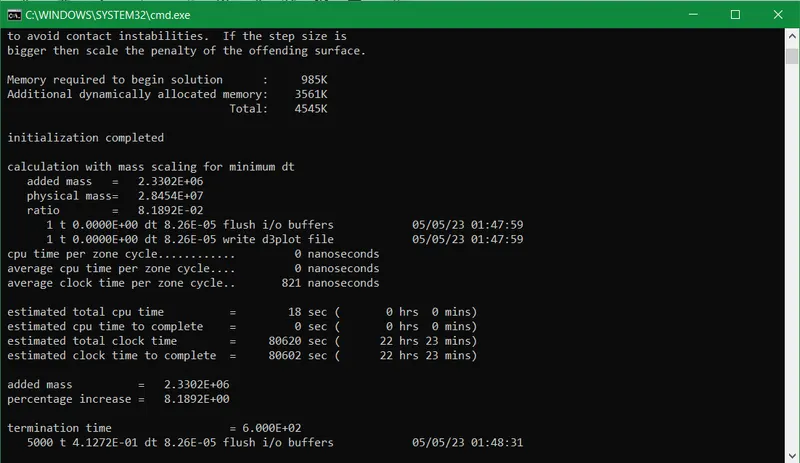
DT2MS -1.100e-04

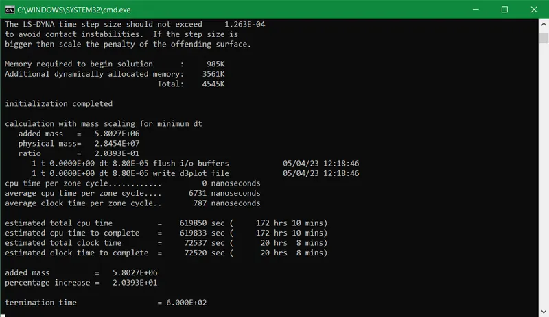
DT2MS -1.500e-04

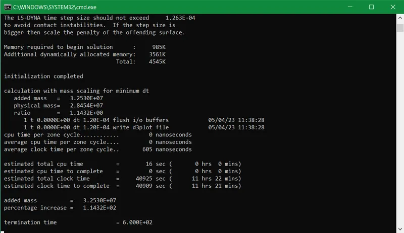
TSSFAC(0.7)

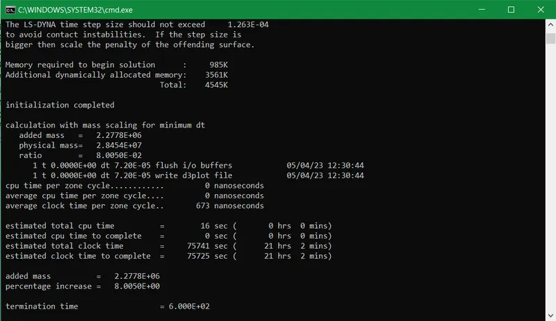
DT2MS -1.029e-04

TSSFAC(0.6)

DT2MS -1.029e-04

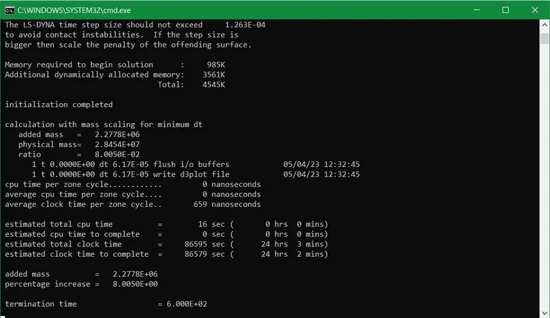
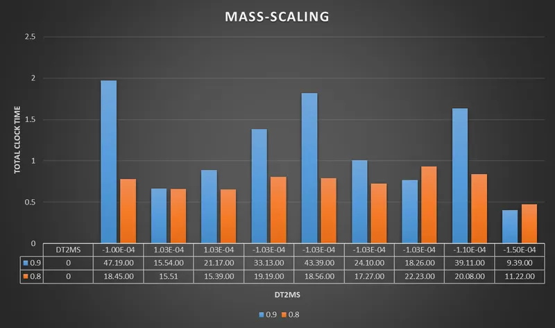
• The total clock time for 0.6 and 0.7 values of TSSFAC keeps on increasing so there is no point in taking them into account. The values beyond 0.9 will create numerical instabilities and 0.67 is usually put as constant. Lastly, we make a comparison for total clock time between 0.8 and 0.9 TSSFAC entities.

IMPLICIT ANALYSIS

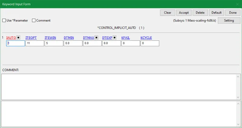
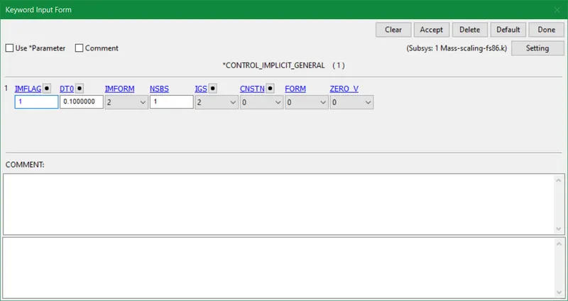
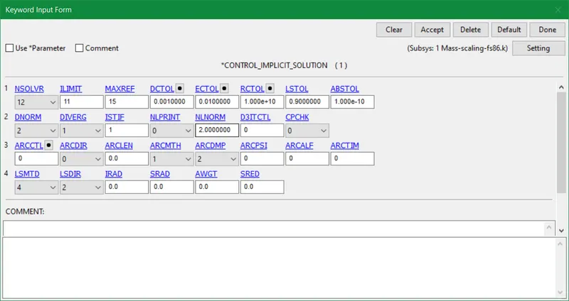
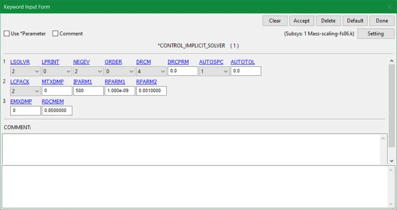
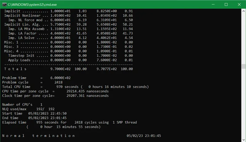
• The control_timestep card doesn't work for the implicit scheme so we delete it or comment on it in the keyword file. The necessary control implicit cards are keyed in this model for implicit analysis as displayed below. However, we save the file, run the simulation and note down the total CPU time of the simulation.

SN0.	SCHEME/ANALYSIS	TOTAL TIME
1.	EXPLICIT	19 HOURS 19 MINUTES
2.	IMPLICIT	16 MINUTES 10 SECONDS

CONCLUSION:

1. Despite the fact the running time for implicit analysis is shorter than that of explicit analysis, this is due to the reason that the timestep in the implicit analysis is larger than in explicit analysis, and we used a constant timestep composition.
2. When DT2MS values for TSSFAC are set to 0.8, they produce a consistently shorter running time than other values.
3. The total clock time taken converges for varied DT2MS values in an explicit analysis while monitoring the graph. It doesn't take a path for constant parameters while regulating time step entries.
4. Iterations are used in the implicit analysis, and mass scaling is not employed. The concept of mass scaling and its importance require explicit analysis.