Week - 10 Hyperelastic Material Models

HYPERELASTIC MATERIAL MODELS

INTRODUCTION

HYPERELASTIC MATERIALS:

The traditional linear-elastic material models do not correctly reflect the observed material behavior for many materials. Rubber is the most typical example of this type of material, with a stress-strain relationship that is non-linearly elastic, isotropic, incompressible, and generally independent of strain rate. Many biological tissues can also be represented as hyperelastic materials.

More advanced models are required for rubbery and biological materials. At small stresses, such materials may display nonlinear stress-strain behavior, whereas, at large strains, they may be elastic. These complicated non-linear stress-strain behaviors must be handled by strain-energy density functions that are properly tuned.
The Neo-Hookean solid is the most basic of these hyperelastic models.

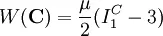
where μ is the shear modulus, which may be measured experimentally. Experiments show that the Neo-Hookean model matches the material behavior with adequate precision for rubbery materials under mild straining up to 30-70%. The one-parametric Neo-Hookean model is substituted by more generic models, such as the Mooney-Rivlin solid, to simulate rubber at high stresses, where the strain energy W is a linear combination of two invariants.

Mooney-Rivlin material was initially designed for rubber, but it is now commonly used to mimic (incompressible) biological tissue.

OGDEN (HYPERELASTIC MODEL):

The more advanced Ogden material model has been created for modeling rubbery and biological materials at even greater stresses. The Ogden material model is a hyperelastic material model that is used to describe the nonlinear stress-strain behavior of complex materials like rubber and biological tissue. The model is based on the idea that the material behavior may be represented by a strain energy density function, from which stress-strain equations can be determined. A strain energy density function is a hyperelastic material model. The function simply connects the energy contained in an elastic material, and hence the stress-strain connection, to the three strain (elongation) components, ignoring deformation history, heat dissipation, stress relaxation, and so on. The Neo-Hookean, Mooney-Rivlin, and Ogden models are examples of strain energy density functions. The Ogden model is frequently used to simulate rubberlike materials like polymers and biological materials. These materials are usually isotropic, incompressible, and strain rate independent.

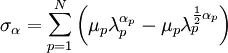
The strain energy density in the Ogden material model is now stated in terms of the primary stretches.

, as:

where N, and are material constants. Under the assumption of incompressibility, one can rewrite as

In general the shear modulus results from

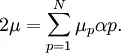
Rubber material behavior may be very well characterized with N = 3 and by fitting the material characteristics. The Ogden model will reduce to either the Neo-Hookean solid (N = 1, = 2) or the Mooney-Rivlin material (N = 2, 1 = 2, 2 = 2) for certain values of material constants.

Using the Ogden material model, the three principal values of the Cauchy stresses can now be computed as

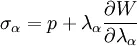
where use is made of

We now consider an incompressible material under uniaxial tension, with the stretch ratio given as .

The principal stresses are given by

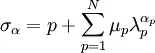
The pressure p is determined from incompressibility and boundary condition σ₂ = σ₃ = 0, yielding:

Many models exist to describe hyperelastic behavior, each starting with a different strain-energy density function. In practice, however, since it combines accuracy with computational simplicity, the Ogden material model has become the reference material law for understanding the behavior of natural rubbers.

AIM

• Given the material data below, calculate the Mooney Rivlin and Ogden material constants and compare both using stress-strain data from a Dogbone specimen tensile test with 100 percent strain.
• The given data is the engineering stress-strain in MPa/(mm/mm).
• The comparison should be shown from the d3hsp file and using simulation.

EXPLANATION

HYPERELASTIC MATERIALS:

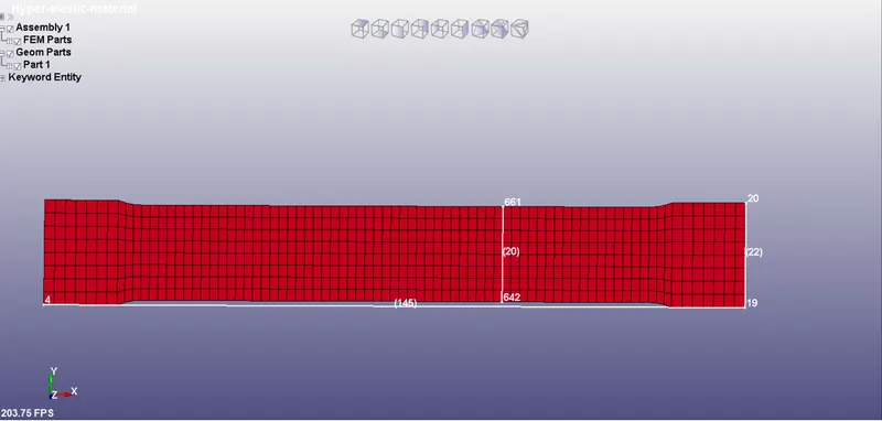
• The dog-bone specimen input model file (.k) is imported into the LS-Dyna for this assignment. In this assignment, the nature of hyperplastic material is studied w.r.t the change in load using a uniaxial test (tensile test). The original length of the specimen prior to post-processing is noted as

L= 145mm

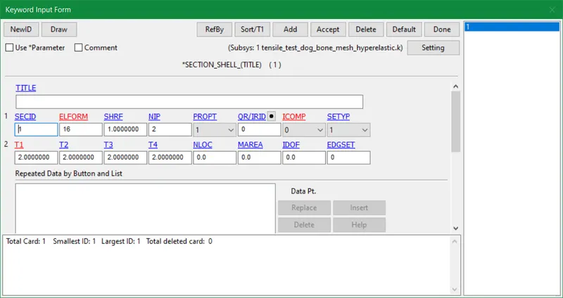
• This is a shell component so we input the section_shell card with desired values. The ELFORM 16 is used because we are employing implicit analysis in this simulation.

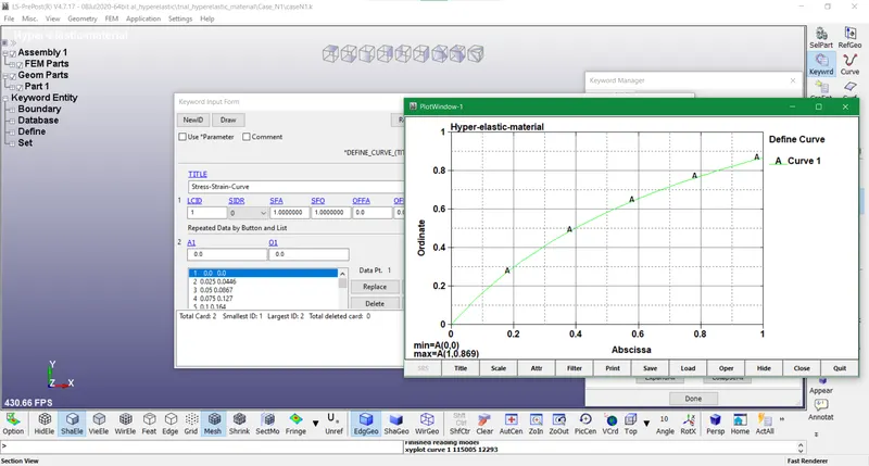
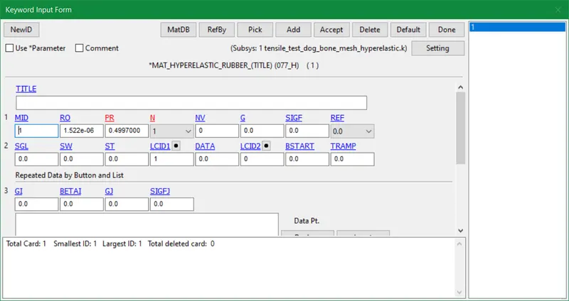
• The provided input Engineering Stress-Strain values are allocated to the load curve ID in the Mat_Hyperelastic_077 card as shown below. The other values computed for this hyperelastic card are

Poisson's ratio, µ = 0.4997

Mass Density, 'rho' = 1522 Kg/m^3

= 1522E-09 Kg/mm^3

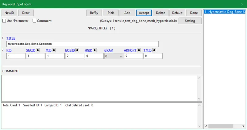
• The boundary conditions are set up after assigning material to this specimen. The prescribed motion (translational) is given towards the x-axis in this model and the other side is constrained in the x-axis. After several failures, we attained a perfect load value i.e. 151 so we inserted the same in the boundary motion card. This load produces a 100% strain rate, and the calculations will be displayed after the simulation results.

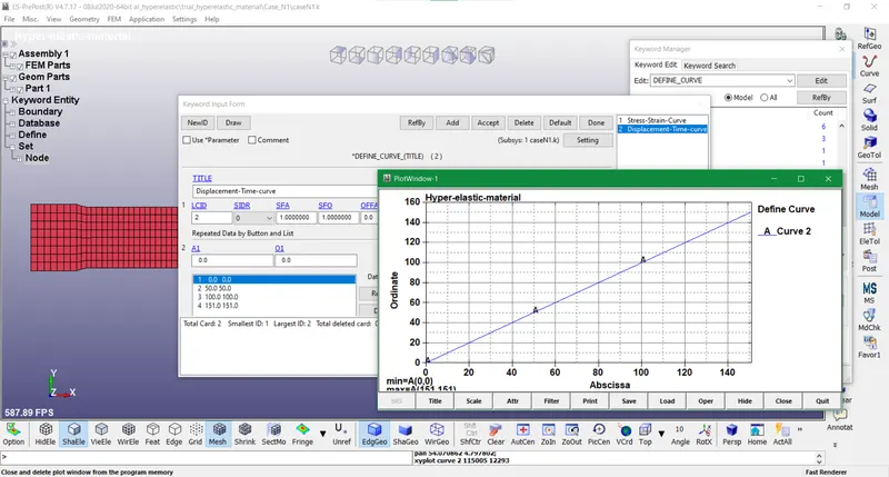
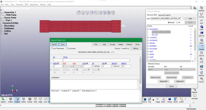
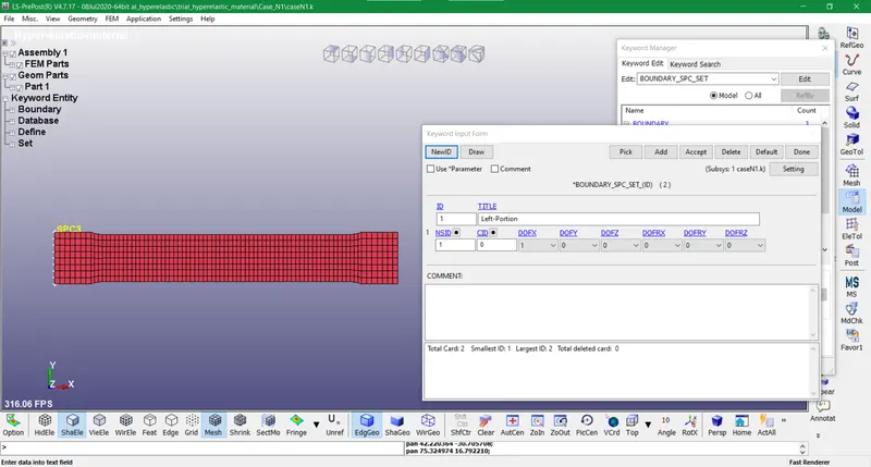
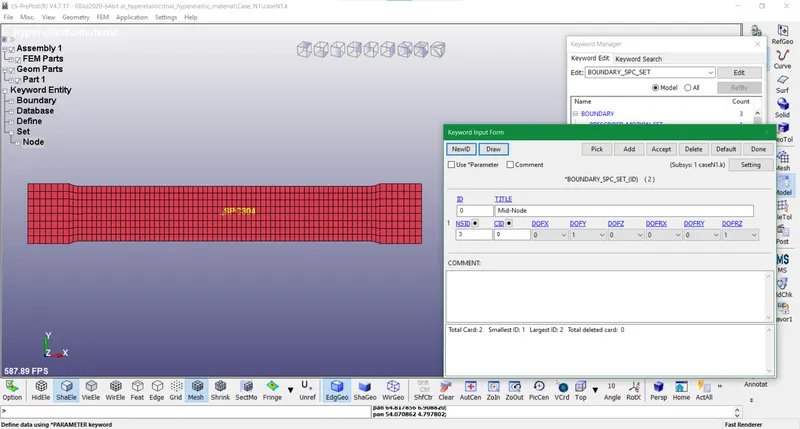
• The implicit cards that are mandatory for this type of simulation are also specified with appropriate figures.

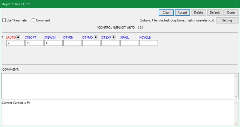
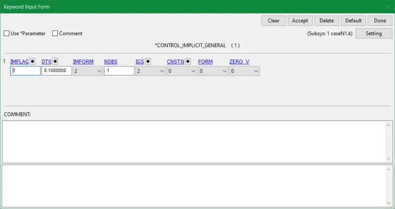
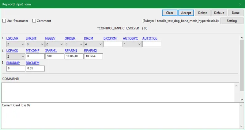
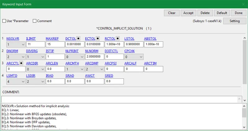
• The termination time and other essential cards that are required to plot energies, stress-strain results so forth, and so on are also placed.

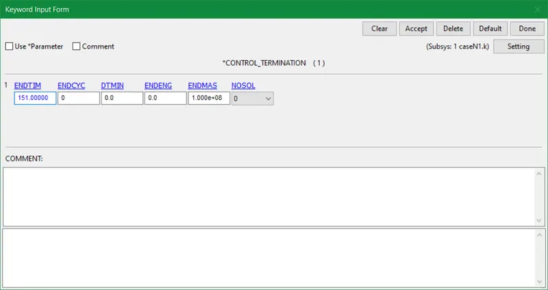
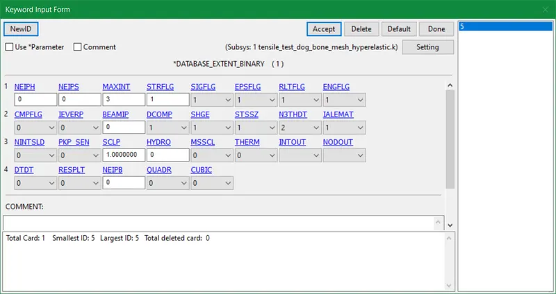
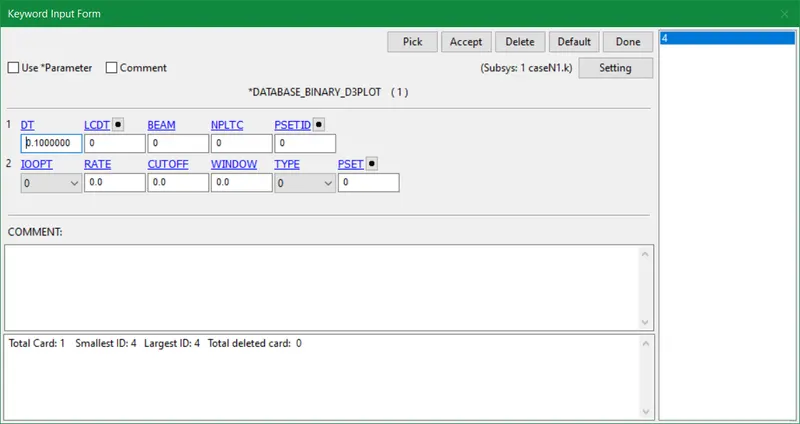
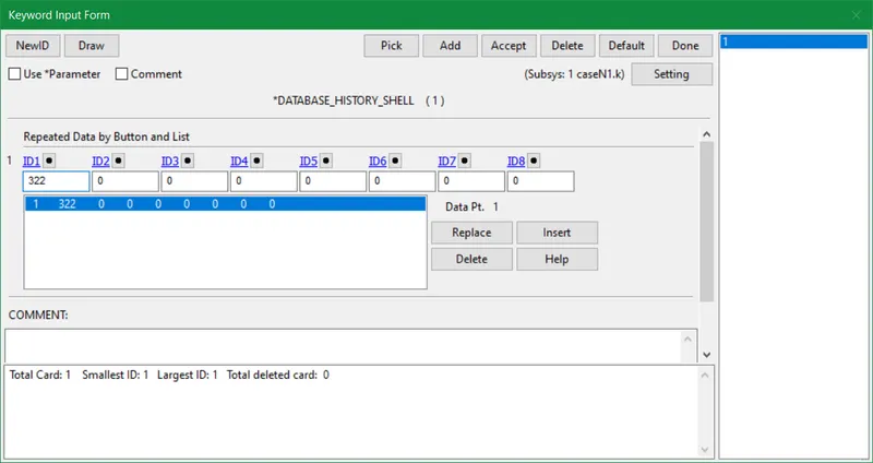
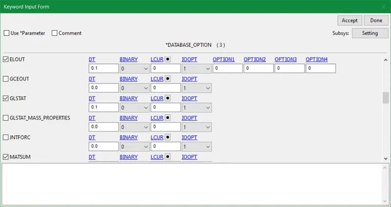
• Lastly, the simulation is started once the model checking is done to make sure there are no errors found.

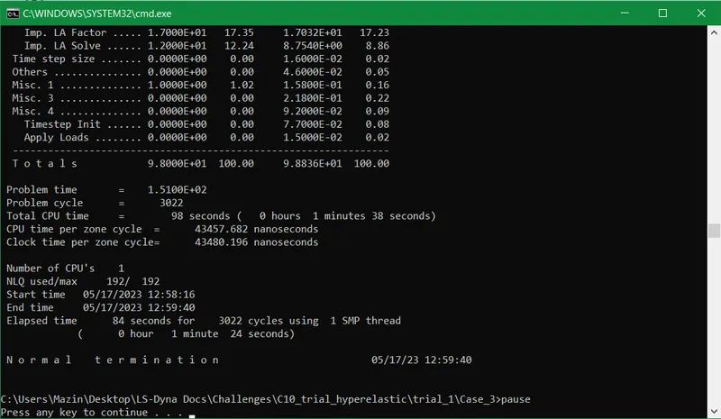
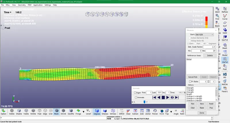
• The simulation file was very large so couldn't upload it but the stress-strain results acquired are portrayed below. Also, the strain rate calculations are also achieved by measuring the final length from the simulation.

Original length L = 145mm

Final length, Lf = 293mm

Strain, e = e=dL/L = (Lf-L)/L = 151/145 = 1 = 100% strain rate

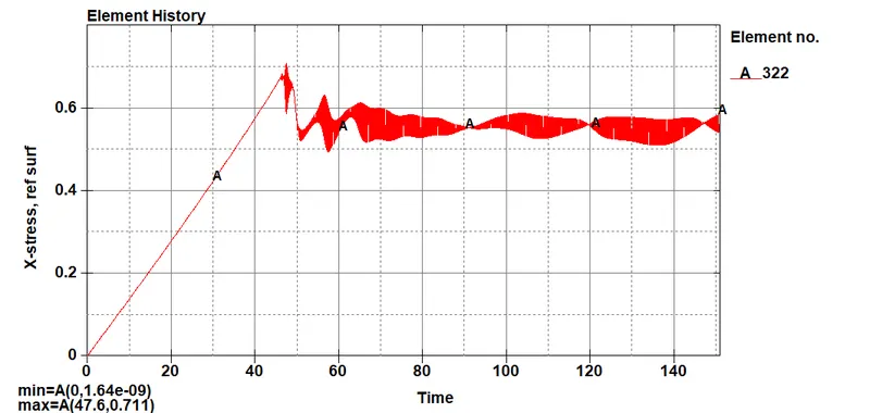
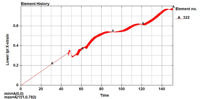
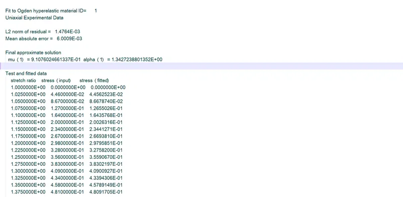
• The D3hsp file obtained post-simulation delivers final stress-strain results and constants.N1, N2, and N3 are only changed in the mat card whilst rerunning the simulation to obtain different results. The final stress and strains can be compared with the original stress strains. The hyperelastic constants are briefly described below:

N Number of hyperelastic constants to solve for from LCID1:
EQ.0: set hyperelastic constants directly.
EQ.1: solve for C10 and C01.
EQ.2: solve for C10, C01, C11, C20, and C02.
EQ.3: solve for C10, C01, C11, C20, C02, and C30.

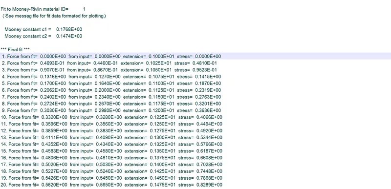
• The calculations for stress-strains and all N constants are computed in an Excel file for hyperelastic material attached to this report.

OGDEN RUBBER MATERIAL:

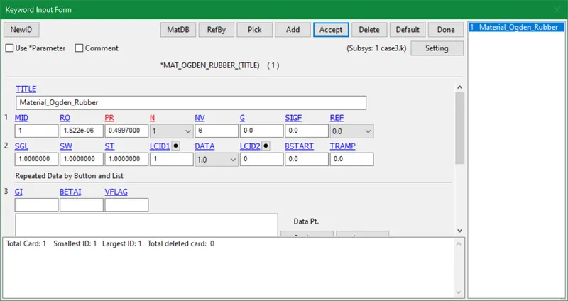
• In the case of Ogden rubber material, we only change the material card to mat_ogden_rubber_077 also it has 8 order of fits instead of constants. The method followed by Ogden Rubber is different as we observe material constants developed post-solving comprised of poisons ratio and principal stretches.

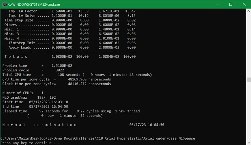
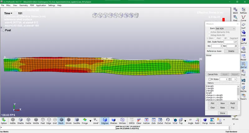
• The strain rate achieved for Ogden material is also 100% after doing the calculations with the final length as 296mm

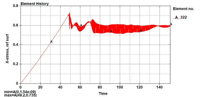
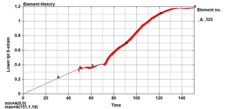
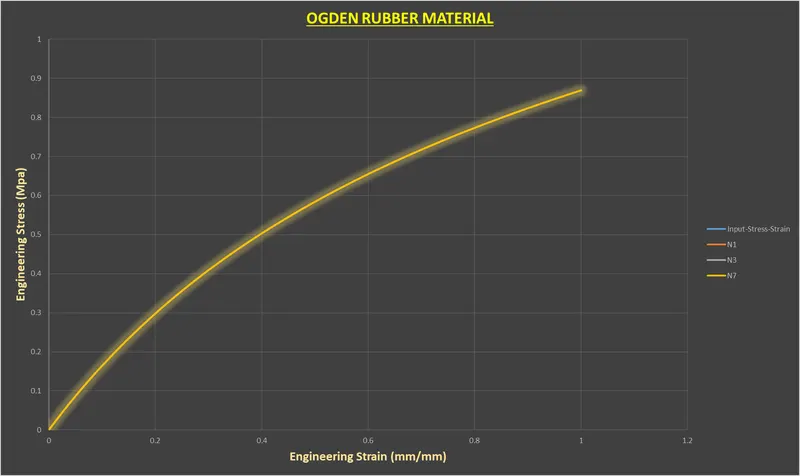
• The stress-strain data of all N material constants for Odgen material is evaluated in the Excel file attached to this report. Also, the stress and strain values attained in Ogden rubber are engineering stress-strain so no need to do conversion unlike in the hyperelastic case.

N = Order of fit to curve LCID1 for the Ogden model, (currently < 9, 2 generally works okay).

CONCLUSION

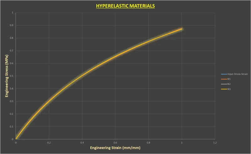
1. The model was basic and didn't have many complications so the results for both cases for all constants contrary to original stress-strain data were uniform.
2. Although we got uniformity throughout the material constants curves of Ogden material superimpose the original material curve. The hyper-elastic material has some minute non-uniformity w.r.t to the original material curve.
3. The Mooney Rivlin N1 curve of the hyper-elastic material was a bit inefficient when compared with any of the curves for Ogden Rubber material constants.
4. Nevertheless, the simulated results demonstrated and verified that when increasing the number of constants the accuracy of the output results also increases.