Assignment 4- To study different material types in Radioss and compare the results.
Objective:- To study different material types in Radioss and compare the results.
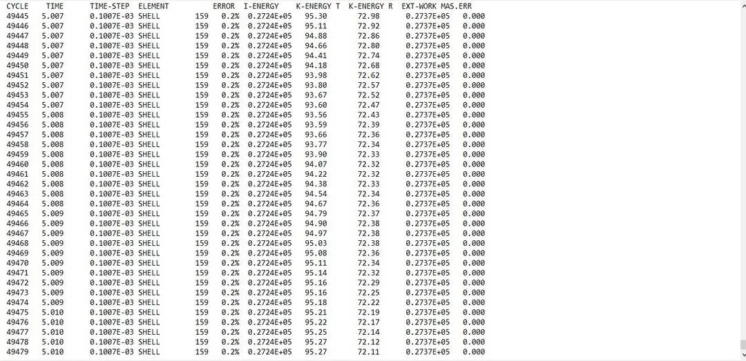
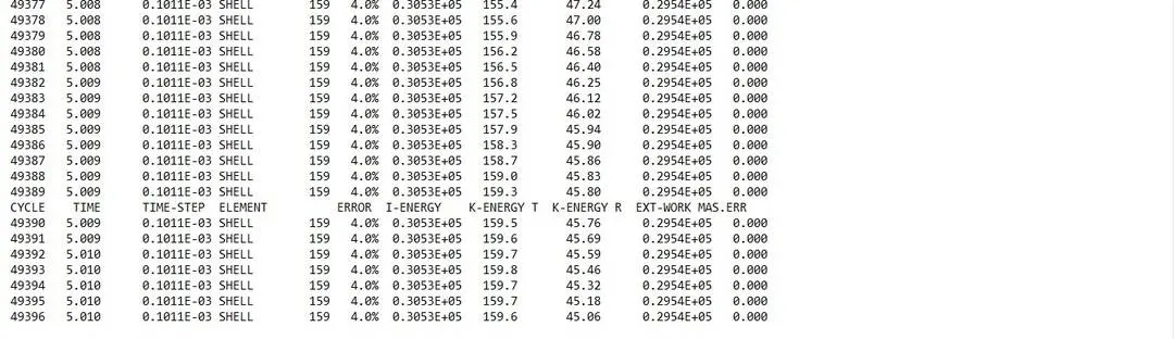
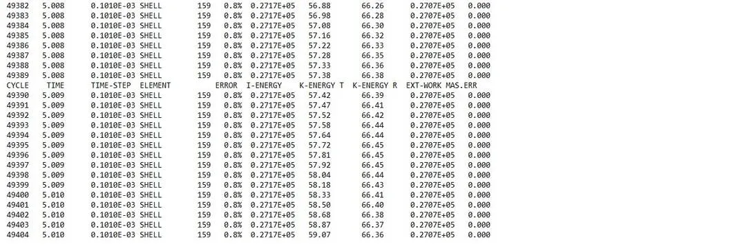
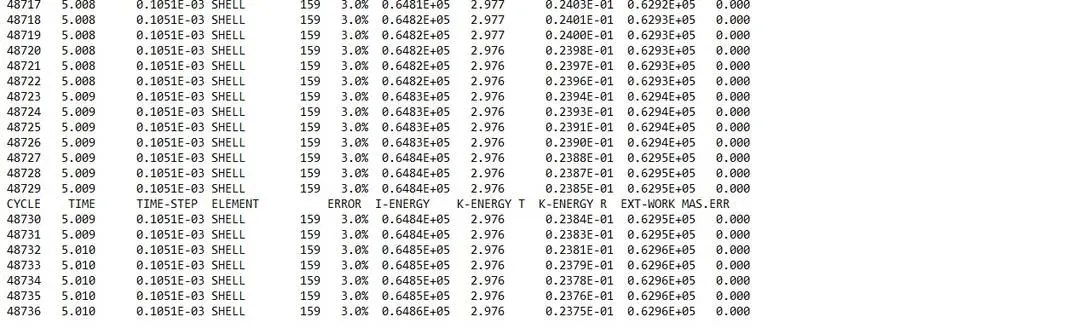
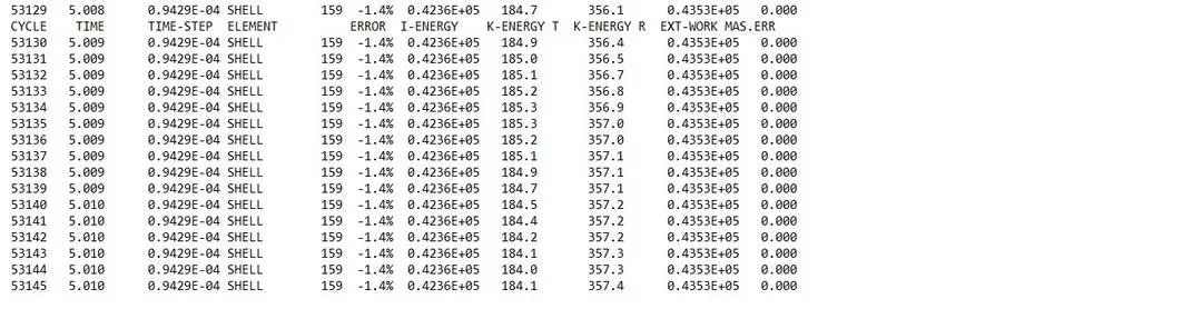
1. The total number of cycles, Energy error, mass error and simulation time.
2. Notice the animation of all 5 and describe the animations in brief on the basis of whether the elements are being deleted or cracked.
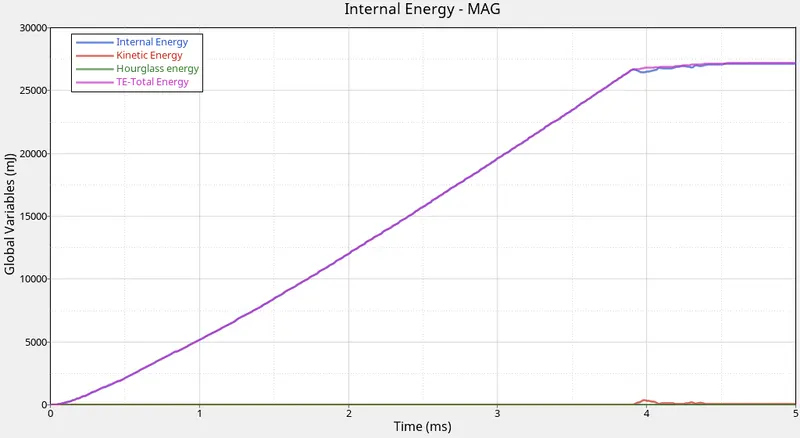
3. Plot energies and notice any difference.
4. Based on all the results, which case would represent the on-field scenario.
5. List down case by case result and your conclusion as to why the failure happened.
LAW 1: Isotropic Elasticity:
This law defines an elastic material using Hooke's law which represents a linear relationship between stress and strain. It is available for truss, beam, shell and solid elements. This material law can only be used for a purely elastic material. This material stiffness is determined by 2 values Young's modulus and Poisson's ratio.
LAW 2: Jhonson-Cook:
This law represents an isotropic elasto-plastic material using the Johnson-Cook material model. This model expresses material stress as a function of strain, strain rate and temperature. A built-in failure criterion based on the maximum plastic strain is available. While using these in FE models, failure of the element happens when 1 integration point reached EPS_max. This means if any of the tension, compression or bending strain value reach the EPS_max, the element fails.
`sigma = (a+b(epsilon^n))(1+cln(epsilon/epsilon_0))(1-T_m)`
where, `(a+b(epsilon^n))` is the influence of plastic strain
`(1+cln(epsi/epsi_0)` is the influence of strain rate
`(1-(T^x)^m)` is the influence of temperature change
The Jhonson - Cook model does not perfectly represent real conditions. It is usually defined using Max stress or strain. A failure law called Jhonson Failure can hence be used to define failure using D1, D2, D3, D4 constants.
LAW 27: Elasto-Plastic material with Brittle Failure:
This law combines an isotropic elasto-plastic Johnson-Cook material model with an orthotropic brittle failure model. Material damage is accounted for prior to failure. Failure and damage occur only in tension. This law is applicable only for shells.
The parameters used to model it are:-
`epsilon_t`= Strain at the beginning of tensile failure
`epsilon_m`= Maximum tensile strain where the stress goes to zero but the element does not fail
`d_max`= Maximum damage factors
`epsilon_f` = Maximum tensile strain for element deletion.
LAW 36: Elastic-Plastic Piecewise Linear:
This law models an isotropic elasto-plastic material using user-defined functions for the work-hardening portion of the stress-strain curve (for example, stress vs. plastic strain) for different strain rates.
In this case, material failures are defined using 4 parameters:
`epsilon`_t= Strain at tensile failure beginning
`epsilon`_m= Strain at which the stress is brought down to zero
`epsilon`_f= Tensile strain for element deletion
`epsilon`_p_max = Maximum strain allowed in compression, tension and bending for element deletion
Procedure:-
CASE 1:- Law2_epsmax_failure
- Open HyperMesh, choose user profile as Radioss and via import solver deck open FAILURE_JOHNSON_0000.rad file.
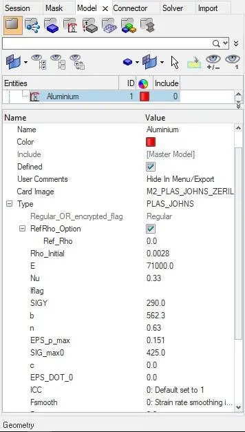
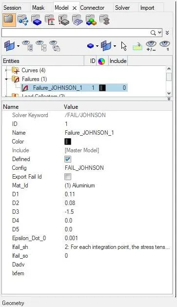
- In this case, the material card is M2_PLAS_JOHNS_ZERIL and the failure card is FAIL_JOHNSON_1.
- Save the file as Law2_epsmax_failure via Eport solver deck.
- Import the Law2_epsmax_failure and under Analysis -> Radioss -> Input = choose where the file will be stored -> Option = -nt 4 -> Radioss.
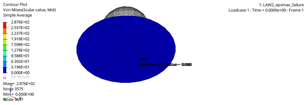
- After running Radioss, open hyperview and load the h3d file obtained, the Von-Mises contour plot can be obtained by select "Contour" -> Result type = Von Mises(s) -> Averaging method = simple -> Apply.
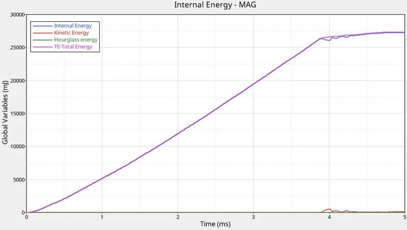
- To obtain the required graphs split the GUI and from "client selector" select HyperGraph 2D and in the data file load the T01 file obtained from simulation also for X type= time, Y type = Global variables, Y request = Internal energy, Kinetic energy, Hourglass energy, Total energy, y component = MAG and click on apply.
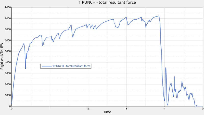
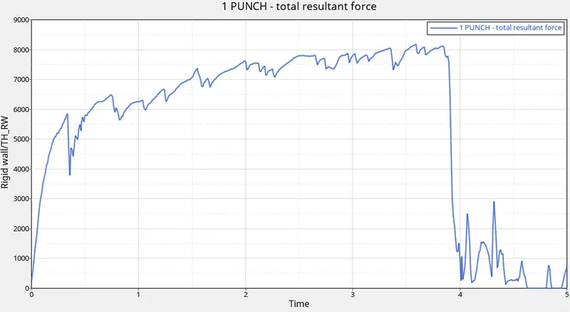
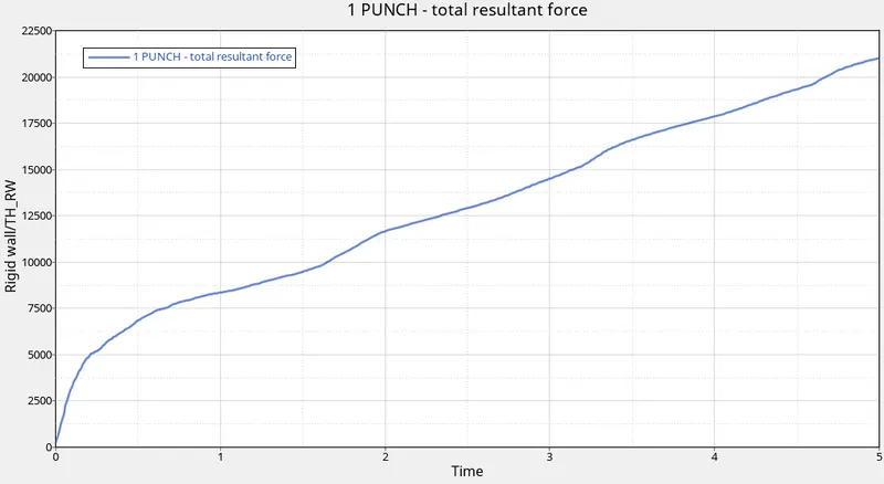
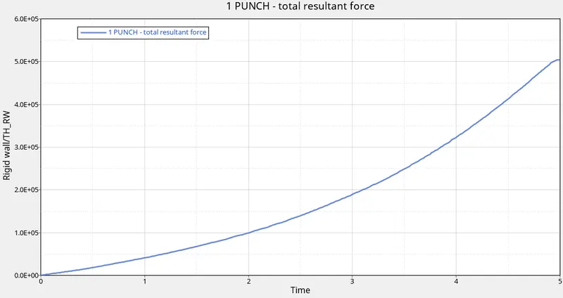
- For the rigid wall forces graphs, X type= time, Y type = Rigid wall/TH_RW, Y request = 1PUNCH, Y component= total resultant force and click on apply.
CASE 2:- Law2_epsmax_crack
- Open HyperMesh, choose user profile as Radioss and via import solver deck open FAILURE_JOHNSON_0000.rad file.
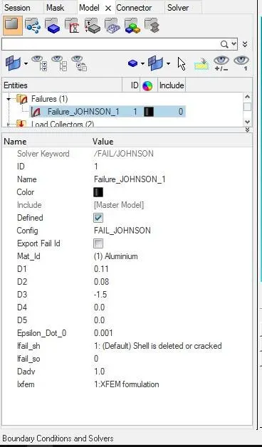
- In this case, change the value of Ifail_sh= 1, Dadv= 1 and Ixfem= 1 in the failure card FAIL_JOHNSON_1.
- Save the file as Law2_epsmax_crack via Eport solver deck.
- Import the Law2_epsmax_crack and under Analysis -> Radioss -> Input = choose where the file will be stored -> Option = -nt 4 -> Radioss.
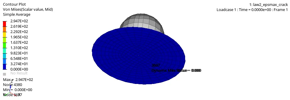
- After running Radioss, open hyperview and load the h3d file obtained, the Von-Mises contour plot can be obtained by select "Contour" -> Result type = Von Mises(s) -> Averaging method = simple -> Apply.
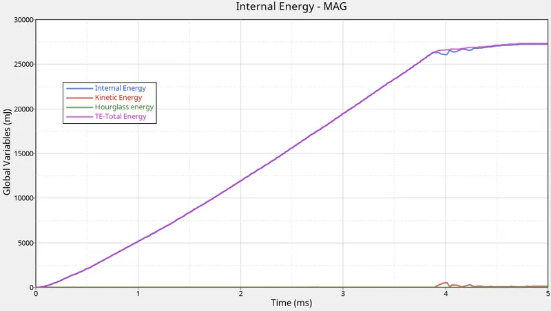
- To obtain the required graphs split the GUI and from "client selector" select HyperGraph 2D and in the data file load the T01 file obtained from simulation also for X type= time, Y type = Global variables, Y request = Internal energy, Kinetic energy, Hourglass energy, Total energy, y component = MAG and click on apply.
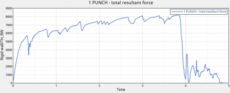
- For the rigid wall forces graphs, X type= time, Y type = Rigid wall/TH_RW, Y request = 1PUNCH, Y component= total resultant force and click on apply.
CASE 3:- Law2_epsmax_nofail
- Open HyperMesh, choose user profile as Radioss and via import solver deck open FAILURE_JOHNSON_0000.rad file.
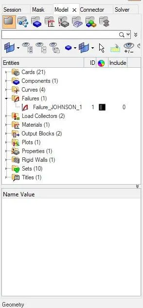
- In this case, delete the failure card FAIL_JOHNSON_1.
- Save the file as Law2_epsmax_nofail via Eport solver deck.
- Import the Law2_epsmax_nofail and under Analysis -> Radioss -> Input = choose where the file will be stored -> Option = -nt 4 -> Radioss.
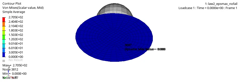
- After running Radioss, open hyperview and load the h3d file obtained, the Von-Mises contour plot can be obtained by select "Contour" -> Result type = Von Mises(s) -> Averaging method = simple -> Apply.
- To obtain the required graphs split the GUI and from "client selector" select HyperGraph 2D and in the data file load the T01 file obtained from simulation also for X type= time, Y type = Global variables, Y request = Internal energy, Kinetic energy, Hourglass energy, Total energy, y component = MAG and click on apply.
- For the rigid wall forces graphs, X type= time, Y type = Rigid wall/TH_RW, Y request = 1PUNCH, Y component= total resultant force and click on apply.
CASE 4:- Law2
- Open HyperMesh, choose user profile as Radioss and via import solver deck open FAILURE_JOHNSON_0000.rad file.
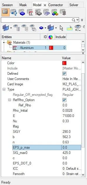
- In this case, under the material delete the value of EPS_p_max and set it to 0, also delete the failure card.
- Save the file as Law2 via Eport solver deck.
- Import the Law2 and under Analysis -> Radioss -> Input = choose where the file will be stored -> Option = -nt 4 -> Radioss.
- After running Radioss, open hyperview and load the h3d file obtained, the Von-Mises contour plot can be obtained by select "Contour" -> Result type = Von Mises(s) -> Averaging method = simple -> Apply.
- To obtain the required graphs split the GUI and from "client selector" select HyperGraph 2D and in the data file load the T01 file obtained from simulation also for X type= time, Y type = Global variables, Y request = Internal energy, Kinetic energy, Hourglass energy, Total energy, y component = MAG and click on apply.
- For the rigid wall forces graphs, X type= time, Y type = Rigid wall/TH_RW, Y request = 1PUNCH, Y component= total resultant force and click on apply.
CASE 5:- Law1
- Open HyperMesh, choose user profile as Radioss and via import solver deck open FAILURE_JOHNSON_0000.rad file.
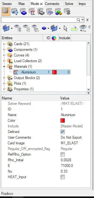
- In this case, under the material change the Card Image to M1_ELAST and provide values for E= 71000, density= 0.0028 and Poisson's ratio= 0.33
- Save the file as Law1 via Eport solver deck.
- Import the Law1 and under Analysis -> Radioss -> Input = choose where the file will be stored -> Option = -nt 4 -> Radioss.
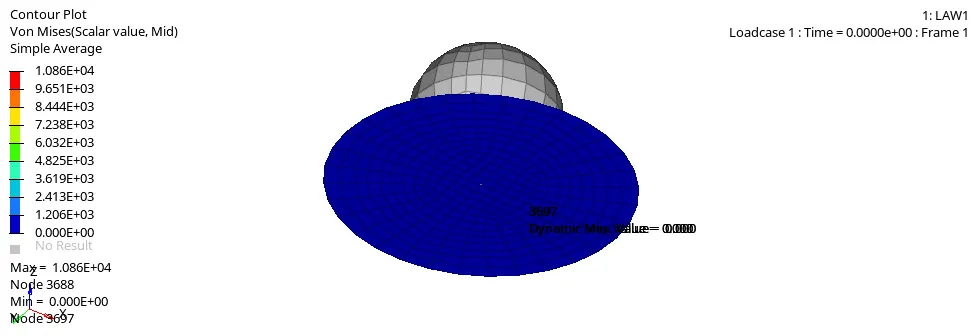
- After running Radioss, open hyperview and load the h3d file obtained, the Von-Mises contour plot can be obtained by select "Contour" -> Result type = Von Mises(s) -> Averaging method = simple -> Apply.
- To obtain the required graphs split the GUI and from "client selector" select HyperGraph 2D and in the data file load the T01 file obtained from simulation also for X type= time, Y type = Global variables, Y request = Internal energy, Kinetic energy, Hourglass energy, Total energy, y component = MAG and click on apply.
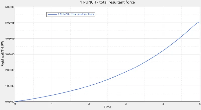
- For the rigid wall forces graphs, X type= time, Y type = Rigid wall/TH_RW, Y request = 1PUNCH, Y component= total resultant force and click on apply.
CASE 6:- Law27
- Open HyperMesh, choose user profile as Radioss and via import solver deck open LAW27_0000.rad file.
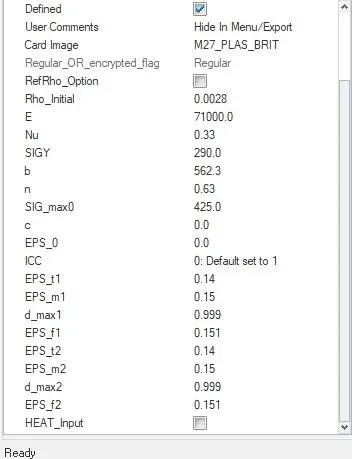
- Check the material card for M27_PLAS_BRIT and recommended values for EPS based failures.
- Run the analysis by, Analysis -> Radioss -> Input = choose where the file will be stored -> Option = -nt 4 -> Radioss.
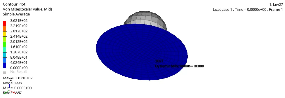
- After running Radioss, open hyperview and load the h3d file obtained, the Von-Mises contour plot can be obtained by select "Contour" -> Result type = Von Mises(s) -> Averaging method = simple -> Apply.
- To obtain the required graphs split the GUI and from "client selector" select HyperGraph 2D and in the data file load the T01 file obtained from simulation also for X type= time, Y type = Global variables, Y request = Internal energy, Kinetic energy, Hourglass energy, Total energy, y component = MAG and click on apply.
- For the rigid wall forces graphs, X type= time, Y type = Rigid wall/TH_RW, Y request = 1PUNCH, Y component= total resultant force and click on apply.
CASE 7:- Law36
- Open HyperMesh, choose user profile as Radioss and via import solver deck open FAILURE_JOHNSON_0000.rad file.
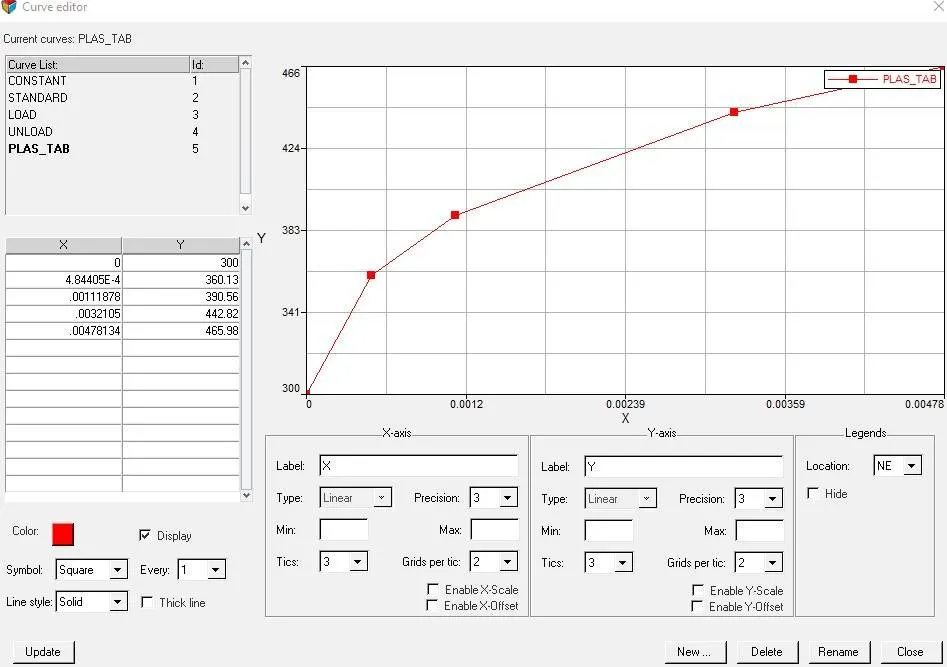
- In this case, under the material change the Card Image to M36_PLAS_TAB and provide values for E= 71000, density= 0.0027, Poisson's ratio= 0.33, EPS_p_max=0.16, EPS_t=0.1 and EPS_m=0.11.
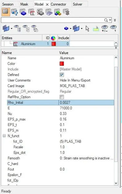
- Before assigning N_funct, create a curve with the given X and Y coordinates and then assign it to the N_funct.
- Save the file as Law36 via Eport solver deck.
- Import the Law36 and under Analysis -> Radioss -> Input = choose where the file will be stored -> Option = -nt 4 -> Radioss.
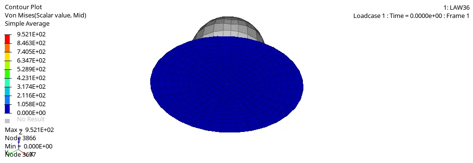
- After running Radioss, open hyperview and load the h3d file obtained, the Von-Mises contour plot can be obtained by select "Contour" -> Result type = Von Mises(s) -> Averaging method = simple -> Apply.
- To obtain the required graphs split the GUI and from "client selector" select HyperGraph 2D and in the data file load the T01 file obtained from simulation also for X type= time, Y type = Global variables, Y request = Internal energy, Kinetic energy, Hourglass energy, Total energy, y component = MAG and click on apply.
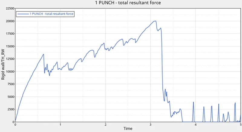
- For the rigid wall forces graphs, X type= time, Y type = Rigid wall/TH_RW, Y request = 1PUNCH, Y component= total resultant force and click on apply.
Comparison:-
| CASE 1 | CASE 2 | CASE 3 | CASE 4 | CASE 5 | CASE 6 | CASE 7 | |
| Type | LAW2_epsmax_failure | LAW2_epsmax_crack | LAW2_epsmax_nofail | LAW2 | LAW1 | LAW27 | LAW36 |
| Failure Configuration | FAILURE_JOHNSON_1 Ifail_sh= 2 | FAILURE_JOHNSON_1 Ifail_sh= 1, Dadv= 1, Ixfem= 1 | Delete FAILURE_JOHNSON_1 | Delete FAILURE_JOHNSON_1, EPS_p_max= 0 | Delete FAILURE_JOHNSON_1 | n/a | Delete FAILURE_JOHNSON_1 |
| Material Card Image | M2_PLAS_JOHNS_ZERIL | M2_PLAS_JOHNS_ZERIL | M2_PLAS_JOHNS_ZERIL | M2_PLAS_JOHNS_ZERIL | M1_ELAST | M27_PLAS_BRIT | M36_PLAS_TAB |
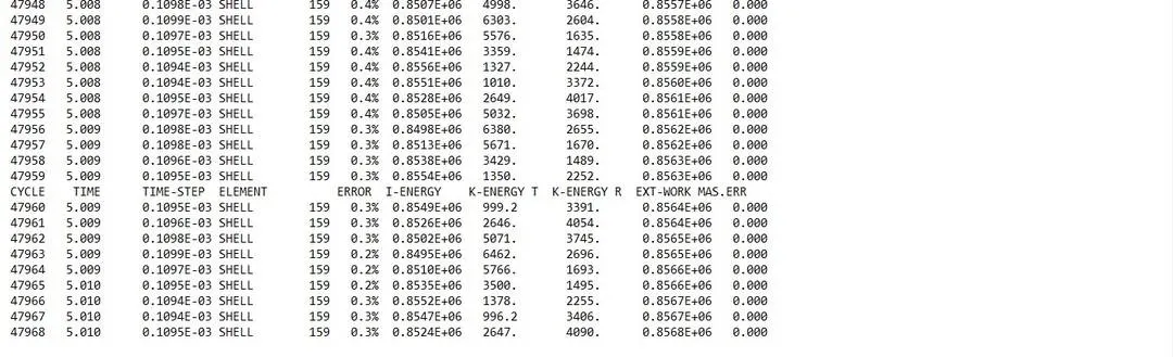
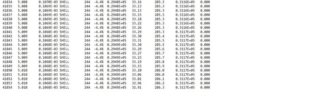
| Energy Error (%) | 0.2 | 4 | 0.8 | 3 | 0.3 | -4.4 | -1.4 |
| Mass Error | 0 | 0 | 0 | 0 | 0 | 0 | 0 |
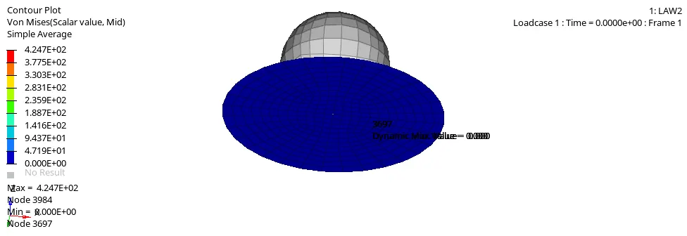
| Max Von Mises Stress | 2.876E+02 | 2.947E+02 | 2.705E+02 | 4.247E+02 | 1.086E+04 | 3.621E+02 | 9.521E+02 |
| Number Of Cycles | 49480 | 49397 | 49405 | 48737 | 47969 | 41855 | 53147 |
| Simulation Time (s) | 128.74 | 132.5 | 128.59 | 126.76 | 132.79 | 109.59 | 153.09 |
- For CASE 1:- When the stress and strain value reach the failure criteria that is 15.1% of plastic strain the elements got deleted but cracking was not observed within those elements.
- For CASE 2:- As Ifail_sh= 1, Dadv= 1 and Ixfem= 1 are set in the FAILURE_JOHNSON_1, where Ixfem helps to decide how to fail the material or element if set to "0" it will delete the element and if set to "1" it will try to break the element as it should have under the given loading condition, so in this case, crack is formation is observed before deletion of the element.
- For CASE 3:- As the FAILURE_JOHNSON_1 card is deleted which means failure mode is not defined therefore the elements gets deleted upon reaching the 15.1% of plastic strain.
- For CASE 4:- As the FAILURE_JOHNSON_1 card is deleted and the EPS_p_max= 0, no elements of the circular plates gets deleted and the plate is showing elastic behaviour.
- For CASE 5:- The material card is M1_ELAST and is defined using Young's modulus, Poison's ratio and density and it defines linear elastic using Hooke's law, therefore, the elements of the plate get stretched behaving like an elastic membrane.
- For CASE 6:- In this case, the material card is set to M27_PLAS_BRIT which shows Elasto-Plastic behaviour with Brittle Failure and the element failure criteria are set in 2 different principal directions, so the elements get deleted as soon as they reached the tensile failure strain value.
- For CASE 27:- In this case, the material card is M36_PLAS_TAB where the stress-strain curve is user-defined so here plastic behaviour is observed and then the failure of the elements.
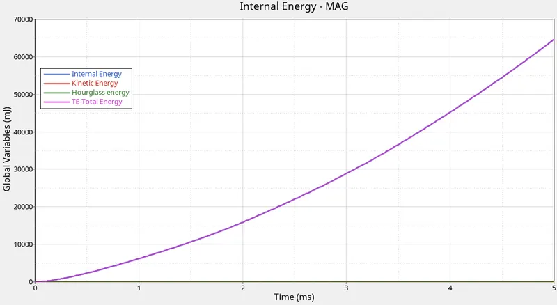
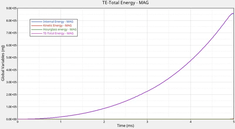
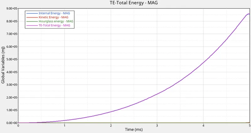
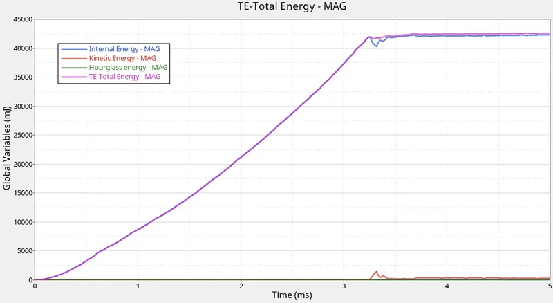
- The energy graph for Case 1, 2 and 3 appear to be somewhat similar but for Case 4 the internal energy and total energy rises exponentially. But in the case of 6 and 7 the internal energy and the total energy increases continuously up to some extent than becomes constant.
Conclusion:
- The best representation for the on-field scenario would be case 7 as it data is more practical in comparison to other cases.
- The hourglass energy remained almost zero in all the cases also the mass error is zero also the energy error is within the limits for all the cases.