Week - 9 Material Modeling from Raw Data

AIM: To Simulate and Validate the curve as shown in the above figure.

KEYWORDS: Dogbone Specimen, Rigid material, tensile, True stress, Engg stress, etc.,

SOFTWARE: LS-Dyna

OBJECTIVE:

1. From the above video link, extract the data from the figure and used it for validation.

2. Using the diagram of the true stress-strain curve given for graphite iron casting, creating a material model for the Dogbone specimen.

3. Validating the material model by performing a tensile test on a Dogbone specimen.

INTRODUCTION:

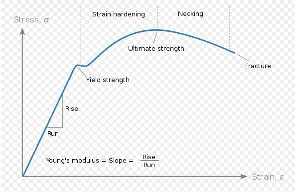
In engineering and materials science, a stress–strain curve for a material gives the relationship between stress and strain. It is obtained by gradually applying a load to a test coupon and measuring the deformation, from which the stress and strain can be determined (see tensile testing). These curves reveal many of the properties of a material, such as Young's modulus, the yield strength, and the ultimate tensile strength. Engineering stress is the applied load divided by the original cross-sectional area of a material. Also known as nominal stress. True stress is the applied load divided by the actual cross-sectional area ( the changing area with respect to time) of the specimen at that load.

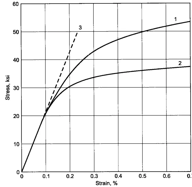
A stress-strain curve for the graphite iron casting is given in the problem statement. Two curves with different material structures have been shown in the figure below. This response should be captured by either MAT_024(Piecewise linear plasticity) or MAT_018(Power law of plasticity) material model according to the problem statement.

MAT_018(Power law of plasticity):

In this material model, the elastoplastic behavior of the material is defined by a power law of hardening. This is an anisotropic material model. The stress-strain relation is defined by the following equation:

σy=kεn

Where,

σy= Yield strength

k = Strength coefficient

ε= Total strain

n = Hardening coefficient

So, the above equation is used to predict the stress-strain behavior of the elastoplastic material. The curvature of the curve after the yield point is highly dependent on the hardening coefficient (n). This is one of the simple models to describe metal plasticity.

MAT_024(Piecewise linear plasticity):

This material model also models the elastoplastic behavior of the material. Here, the material behavior can be treated as a bi-linear stress-strain curve or can be treated as a multi-linear curve by defining a set of stress-strain points. The multi-linear behavior can also be treated by defining a load curve in terms of effective stress vs effective plastic strain. The basic input material parameters for this model are mass density, yield stress, Poisson's ratio, Young’s modulus, and tangent modulus. The Bi-linear stress-strain curve is the simplest form of representation but the multi-linear curve captures the behavior more accurately. So, the basic concept here is the continuous smooth stress-strain curve is approximated with small linear steps.

Procedure:

1. Data Extraction:

1) The given image file of the true stress-strain graph of graphite iron casting is opened in data digitizer software to extract the data and export it as an excel file. Curve 1 is taken and the data points are selected then, the data is extracted as an excel file.

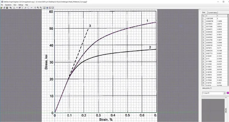
2) For the Material card model we are using the SI unit i.e Kg/mm/ms but if we noticed from the Stress and Strain graph units are give in Ksi and percentage respectively so the unit of stress has to be changed from Ksi to GPa and Strain has to change from percentage to actual value.

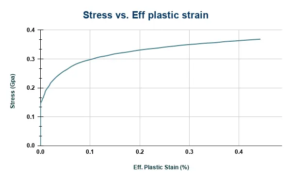
3) The stress-strain data file obtained from the data digitizer is opened in excel to plot a graph of true stress, (GPa) vs true strain as shown in the below first graph. We calculate the Effective Plastic Strain from the true stress and true strain values then, from the second graph shown below, the yield stress value is taken as 0.151 GPa, and the region beyond is considered as the plastic region.

2. Part definition:

1) The material card chosen is MAT_24_PIECEWISE_LINEAR_PLASTICITY to define the behavior of an elastoplastic material with arbitrary stress versus strain curve and arbitrary strain rate dependency. With this material model, it is possible to consider the effect of the strain rate.

The values of density and Poisson’s ratio is taken as generic values.

The given value of young’s modulus = 20.9E+06 psi = 144.1004 GPa.

The yield stress value from the graph = 0.151 GPa.

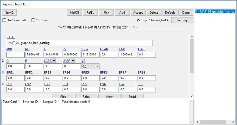
2) The plastic behavior of the material is defined using the LCSS curve option in the material card. The curve is defined by inputting the values of effective plastic strain and effective stress (true stress).To define the LCSS curve the stress values beyond the yield stress values are considered.

The Effective Plastic Strain = True Strain – (True Stress/Young’s Modulus).

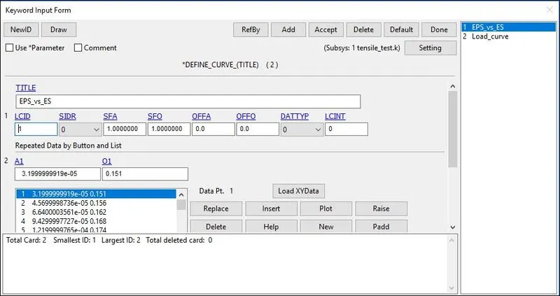
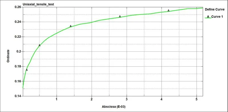
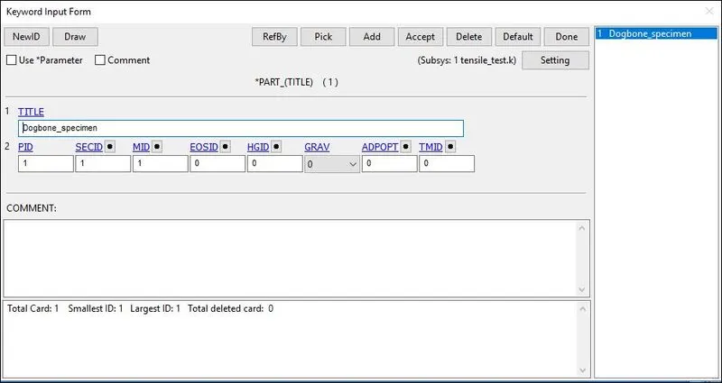
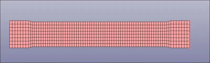
3) The section property of the dogbone specimen is assigned as a shell element with 2 mm thickness and ELFORM=16.

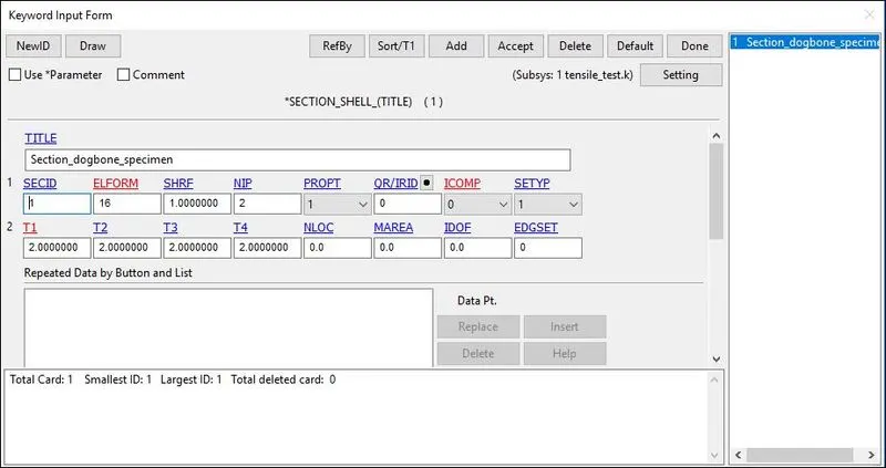
4) The material and section defined are then referenced to the dogbone specimen part.

3. Boundary Condition:

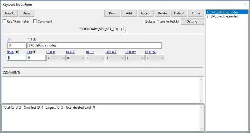
1) The nodes at the fixed end is constrained in the X and Z direction only and the Y direction is not constrained because of lateral expansion during the tensile test.

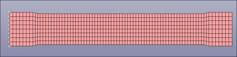
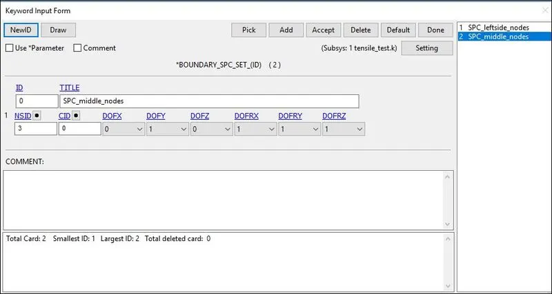
2) The nodes at the middle is constrained in the Y direction since the neutral axis passes through the middle of the specimen in the X-direction.

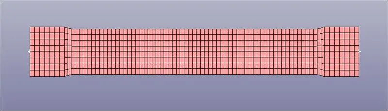
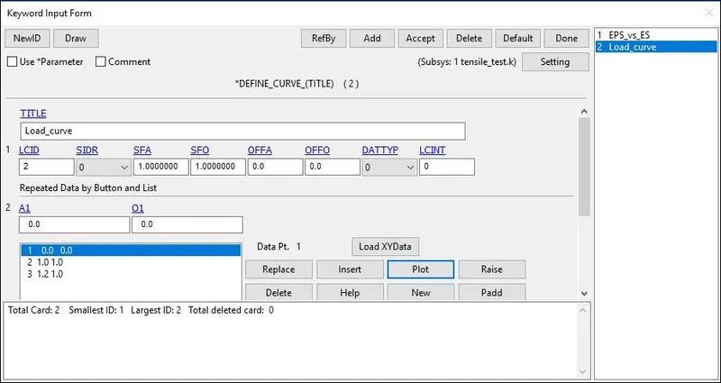
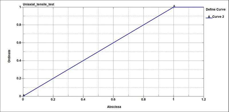
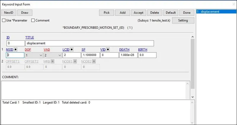
3) The nodes of the pulling end are assigned with a boundary prescribed motion in X direction using a displacement load curve as shown in the below figure.

4. Control cards:

1) The tensile test of a given dogbone specimen is considered as quasi-static analysis, hence implicit analysis is carried out with necessary control implicit cards.

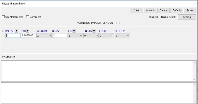
1.*CONTROL_IMPLICIT_GENERAL:

Activate implicit analysis and define associated control parameters. This keyword is required for all implicit analyses

• IMFLAG: Implicit/Explicit analysis type flag: 1- implicit analysis.
• DT0: Initial time step size for implicit analysis: 0.0050000
• IMFORM: Element formulation flag for seamless spring back: 2 retain original element formulation (default).

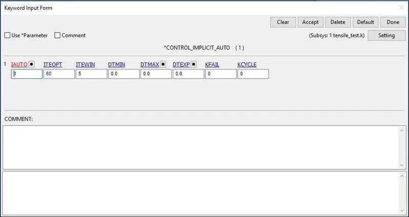
2.*CONTROL_IMPLICIT_AUTO:

This card has been defined to adjusts the time step size

• IAUTO: set to 1 which automatically adjusts the timestep size.
• ITEOPT: optimizes the operation count step:60
• ITEWIN: is the iteration window: 5
• DTMIN: Minimum allowable time step size: 0
• DTMAX: Maximum allowable time step size:0

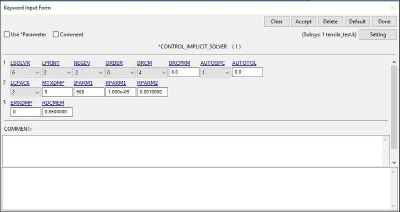
3.*CONTROL_IMPLICIT_SOLVER:

The linear equation solver performs the CPU-intensive stiffness matrix inversion

• LSOLVR: Linear equation solver method: 4 (double-precision solver).

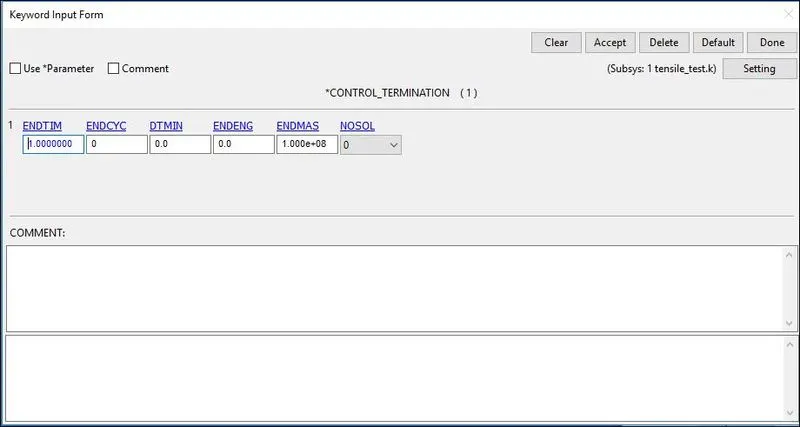
4. *CONTROL_TERMINATION:

This card is used to mention the termination time of the simulation.

• ENDTIM: 1 (Termination time)

5. Database Cards:

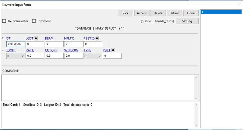
*BINARY_D3PLOT: It defines the frequency at which the animation file is to be created and is set to 0.01 ms

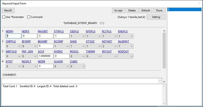
*DATABASE_EXTEND_BINARY: This writes the strain tensor to d3plot when STRFLG is set to 1

*DATABASE_ASCII_Option: The output request in ASCII format, The following keyword is Activated and

1. ELOUT: Element Output Data and
2. GLSTAT: Global Data.

RESULTS & DISCUSSION:

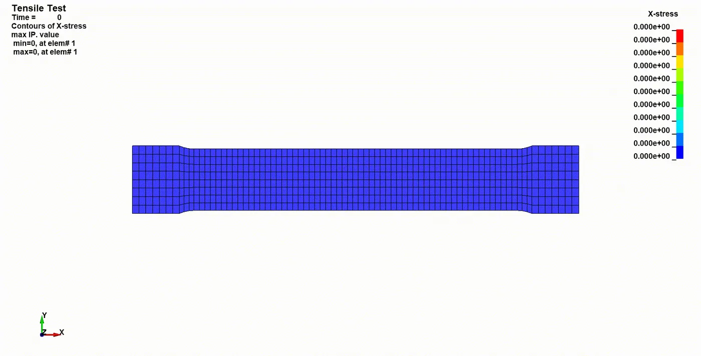
CONTOUR PLOTS FOR X-STRESS:

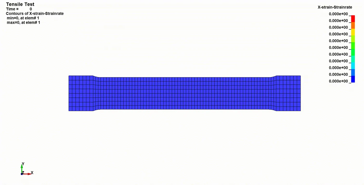
CONTOUR PLOTS FOR X-STRAIN:

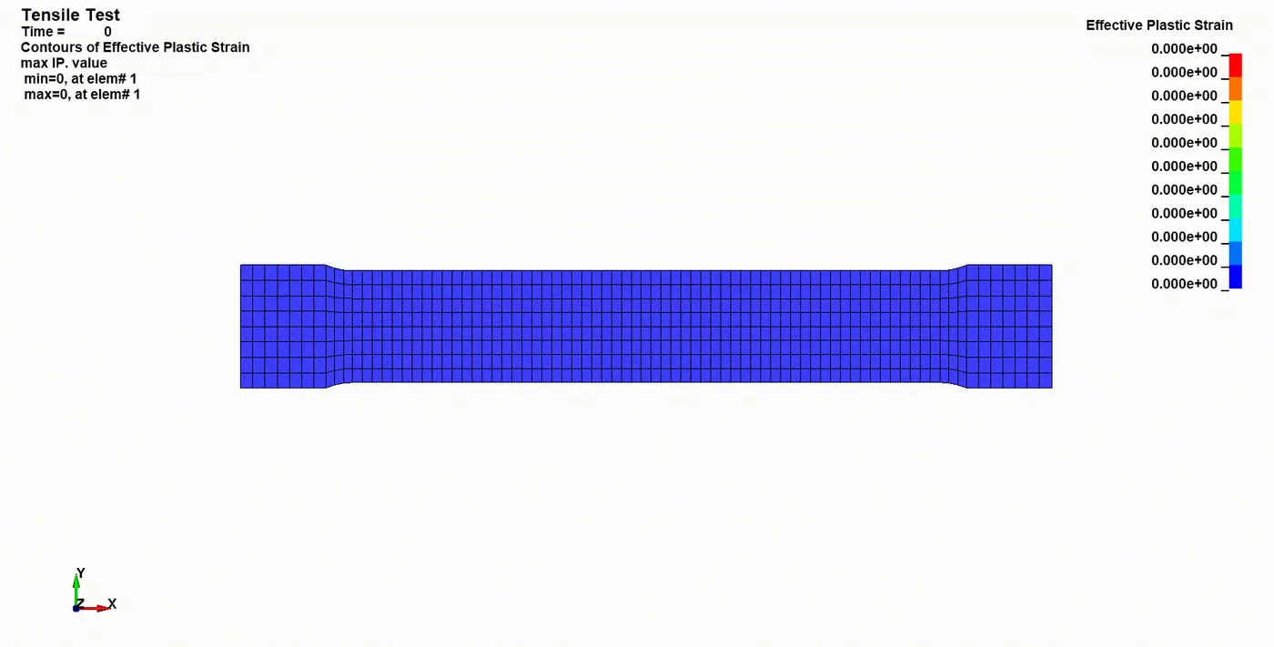
CONTOUR PLOTS FOR EFFECTIVE PLASTIC STRAIN:

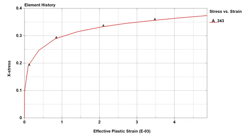
3. Stress vs Strain Plot after simulation:

The true stress vs true strain plot obtained from the simulation of tensile test on dogbone specimen is as shown in the image given below which resembles the given true stress vs true strain plot.

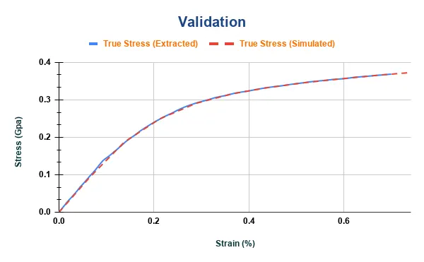
4. Comparison:

Material defined stress-strain data and simulated stress-strain data are compared. It can be seen that the elastic part is linear. The linear elastic part is calculated directly through the given young’s modulus and yielding starts after the first defined yield point in the hardening curve.

CONCLUSION:

1) The stress-strain data extracted from the image is validated with the MAT_024(Piecewise linear plasticity) material model.

2) The stress-strain behaviour after yielding is considered by a hardening curve which is given as an input through the MAT_024 card.

3) The MAT_024 material model captures the actual stress-strain behaviour similarly and almost matched the defined stress-strain curve in the material model.

4) Also we have seen little variation in the simulation data, which can due to the lack of information like density and Poisson’s ratio for the raw data, Mesh Size of the model or defining proper strain rate. These variations can be fine-tuned by trying different values of these properties and by selecting more data points to better capture the curve feature.

NOTE: Please open the "SLX" file in google sheet, WPS format will not take scale factor.