Week - 2 - Explicit and Implicit Analysis
AIM: To Calculate the given equation by using the Explicit and Implicit methods.
KEYWORDS: Nonlinear analysis, load control, Explicit, Implicit, Newton-Raphson, Taylor Series, etc.,
INTRODUCTION:
The finite element method (FEM) is a numerical problem-solving methodology commonly used across multiple engineering disciplines for numerous applications such as structural analysis, fluid flow, heat transfer, mass transport, and anything existing as a real-world force. This practice systematically yields equations and attempts to approximate the values of the unknowns. This method subdivides the overall problem into simpler sub-issues that are easier to solve. In turn, these sub-issues called finite elements to require implicit and/or explicit analysis.
Explicit and implicit methods are approaches used in numerical analysis for obtaining numerical approximations to the solutions of time-dependent ordinary and PDE, as is required in computer simulations of a physical process. Explicit methods calculate the state of a system at a later time from the state of the system at the current time, while implicit methods find a solution by solving an equation involving both the current state of the system and the later one. Mathematically, if Y (t) is the current system state and Y(t+△t) is the state at the later time △t is a small-time step).
Implicit methods require an extra computation (solving the above equation), and they can be much harder to implement. Implicit methods are used because many problems arising in practice are stiff, for which the use of an explicit method requires impractically small time steps △t to keep the error in the result bounded. For such problems, to achieve given accuracy, it takes much less computational time to use an implicit method with larger time steps, even taking into account that one needs to solve an equation of the form at each time step. That said, whether one should use an explicit or implicit method depends upon the problem to be solved.
Calculation:
( I ) Explicit Analysis Method:
f(u) = u³ + 9u² + 4u .................(1)
From (1) it follows that the stiffness of the bar is,
k(u) = dF/du = 3u² + 18u + 4
For this example, three equal load increments (or steps) of ∆F = 1 unit each are used to load the tension bar. The variables used are u for displacement, f for internal force in the bar, F for the external force applied to the bar, and k for stiffness. Incremental displacements or incremental externally applied forces are represented as ∆u or ∆F, respectively. Use is made of the relationship ∆F = k∆u. The analysis proceeds as follows:
Step 1:
u0 = 0
k(u0) = 3u² + 18u + 4
= 0+0+4
k(u0) = 4
∆F = 1
∆u1 = ∆F/k(u0) = 1/4 = 0.25
u1 = u0 + ∆u1 = 0+0.25 = 0.25
Step 2:
k(u1) =3u² + 18u + 4
k(u1) = 8.6875
∆F = 1,
∆u2 = ∆F/k(u1) = 1/8.6875 = 0.1151
u2 = u1 + ∆u2 = 0.25 + 0.1151 = 0.365
Step 3:
k(u2) = 3u² + 18u + 4
k(u1) = 10.9696
∆F = 1
∆u3 = ∆F/k(u2) = 1/10.9696 = 0.09116
u3 = u2 + ∆u3 = 0.365 + 0.09116 = 0.456
Finally, from the three steps the following results are obtained.
External Force,
F_ext = ∆F + ∆F + ∆F = 3.0
Internal Force,
f_int = u³ + 9u² + 4u = 3.79
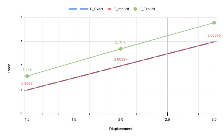
It is evident from the results that external and internal forces are NOT in equilibrium because F_ext ≠ f_int.
| Step | ∆F_i | ∆u_i | u_i | F_ext | f_int | R = f_int - F_ext |
| 1 | 1 | 0.25 | 0.25 | 1 | 1.578 | 0.578 |
| 2 | 1 | 0.115 | 0.365 | 2 | 2.7076 | 0.707 |
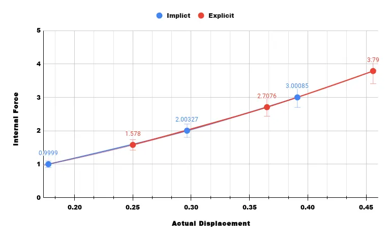
| 3 | 1 | 0.0911 | 0.456 | 3 | 3.790 | 0.790 |
Table_1: Summarizes the main results for the explicit analysis
( II ) Implicit Analysis Method:
f(u) = u³ + 9u² + 4u .................(2)
From (2) it follows that the stiffness of the bar is,
k(u) = dF/du = 3u² + 18u + 4
An implicit analysis is the same as an explicit analysis, except that at the end of each step Newton-Raphson iterations are used to enforce equilibrium before moving to the next step. the following correction is obtained
δuj+1 = -[k(uj)]^(-1) * Rj ................(3)
Notice that the iteration variable is j and it may take several iterations for the norm of the residual 'R' to be reduced below the chosen tolerance criteria (for the example below a tolerance of 10^-2 is chosen).
Step 1:
u0 = 0
k(u0) = 3u² + 18u + 4
= 0+0+4
k(u0) = 4
∆F = 1
∆u1 = ∆F/k(u0) = 1/4 = 0.25
u1 = u0 + ∆u1 = 0+0.25 = 0.25
Check the residual,
F_ext = ∆F = 1
f_int = u³ + 9u² + 4u = 1.578
R(0) = f_int - F_ext = 0.578 > 10^-2, Newton-Raphson iterations are necessary
Calculate the correction to u1 = u1_(0)
δu(1) = -[k(u1_(0)]^(-1) * R(0)
= -8.4^-1 * 0.578
δu(1) = -0.0665
The updated value of u1_(1) = u1_(0) + δu(1)
= 0.25 - 0.0665
u1_(1) = 0.1835
Check the residual again,
F_ext = ∆F = 1
f_int = u³ + 9u² + 4u = 1.0433
R(1) = f_int - F_ext = 0.0433 > 10^-2, Newton-Raphson iterations are necessary
Calculate the correction to u1 = u1_(1)
δu(2) = δu(1) - [k(u1_(1)]^(-1) * R(1)
= -0.0665 - [0.135*0.0433]
= -0.0723
The updated value of u1_(2) = u1_(0) + δu(2)
= 0.25 - 0.0723
u1_(1) = 0.1776
Check the residual again,
F_ext = ∆F = 1
f_int = u³ + 9u² + 4u = 0.9999
R(1) = f_int - F_ext = 0.00012 < 10^-2, Newton-Raphson iterations are not necessary
So the value of u1 = 0.1776
Step 2:
k(u1) =3u² + 18u + 4
k(u1) = 7.2914
∆F = 1,
∆u2 = ∆F/k(u1) = 1/7.2914 = 0.1371
u2 = u1 + ∆u2 = 0.1776 + 0.1371 = 0.3147
Check the residual,
F_ext = ∆F+∆F = 2
f_int = u³ + 9u² + 4u = 2.1813
R(0) = f_int - F_ext = 0.1813 > 10^-2, Newton-Raphson iterations are necessary
Calculate the correction to u2 = u2_(0)
δu(1) = -[k(u2_(0)]^(-1) * R(0)
= -9.962^-1 * 0.1813
δu(1) = -0.0182
The updated value of u2_(1) = u2_(0) + δu(1)
= 0.3147 - 0.0182
u2_(1) = 0.2965
Check the residual again,
F_ext = ∆F+∆F = 2
f_int = u³ + 9u² + 4u = 2.00327
R(1) = f_int - F_ext = 0.0033 < 10^-2, Newton-Raphson iterations are not necessary
So the value of u2 = 0.2965
Step 3:
k(u2) = 3u² + 18u + 4
k(u2) = 9.6
∆F = 1
∆u3 = ∆F/k(u2) = 1/9.6 = 0.1042
u3 = u2 + ∆u3 = 0.2965 + 0.1042 = 0.4006
Check the residual,
F_ext = ∆F+∆F+∆F = 3
f_int = u³ + 9u² + 4u = 3.111
R(0) = f_int - F_ext = 0.1110 > 10^-2, Newton-Raphson iterations are necessary
Calculate the correction to u3 = u3_(0)
δu(1) = -[k(u3_(0)]^(-1) * R(0)
= -9.962^-1 * 0.1110
δu(1) = -0.0095
The updated value of u3_(1) = u3_(0) + δu(1)
= 0.4006 - 0.0095
u3_(1) = 0.3911
Check the residual again,
F_ext = ∆F+∆F+∆F = 3
f_int = u³ + 9u² + 4u = 3.00085
R(1) = f_int - F_ext = 0.00085 < 10^-2, Newton-Raphson iterations are not necessary
So the value of u3 = 0.3911
| Step | ∆F_i | δu_i | u_i | F_ext | f_int | R = f_int - F_ext |
| 1 | 1 | -0.0723 | 0.1776 | 1 | 0.9999 | 1.2e-4 |
| 2 | 1 | -0.0182 | 0.2965 | 2 | 2.00327 | 3.27e-3 |
| 3 | 1 | -0.0095 | 0.3911 | 3 | 3.00085 | 8.5e-4 |
Table_2: Summarizes the main results for the implicit analysis
RESULTS:
(i) Comparison of Force vs Actual displacement of Implicit and Explicit method analysis
(ii) Comparison of Force vs Displacement of Implicit, Explicit & Exact solution