Bird Strike - Project - 2

AIM: To Simulate the Birdstrike on Aero-engine using Explicit Analysis in LS-Dyna.

KEYWORDS: Include, Elastic, Non-Linear Plasticity, Boundary conditions, Elform, etc.,

SOFTWARE: LS-Dyna

OBJECTIVES:

1. The given file contains all the 4 parts which as to separate and save part wise.

2. The suitable material is to be created and saved in a subfolder.

3. The node number, Element number, and parts number are assigned as mentioned above.

4. Create the main file that should have only the *include file and run the explicit simulation.

5. Study the mass scaling by changing the DT2MS.

INTRODUCTION:

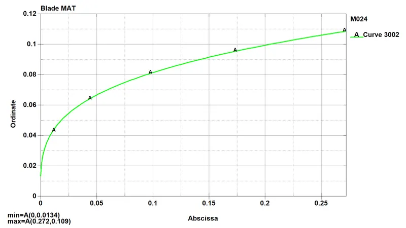
Here, the meshed model of Aero-engine is given which is to be separated as per the above condition. This is a classic nonlinear transient dynamics problem similar to a car crash and mobile drop simulation. This problem can be solved using a generic explicit solver. The blades should rotate at a constant velocity but the casing should remain stationary. Here, the boundary condition is applied for casing so that it should not move in any direction. The cylindrical bird model should travel along its own axis and hit the blades hence velocity is given and assigned in a particular direction and constrained in all directions. For elastic material, Young's modulus for the bird(2000MPa) and the casing(200GPa) are given. The material model for the blades is given as M024 i.e., MAT_PIECEWISE_LINEAR_PLASTICITY. The velocity of the engine blades and the birds can be chosen so that blade failure can be seen within a short span of time. The material for the bird part is considered according to the literature. After all the conditions applied, create the main file and use the *INCLUDE command to involve all the parameters and run the simulation.

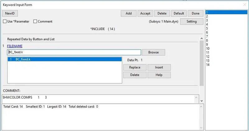
Mass Scaling:

Mass-scaling is a term that is used for the process of scaling the element’s mass in explicit simulations to adjust its timestep. The primary motivation is to change (usually increase) the global compute timestep which is limited by the Courant’s stability criteria. LS-DYNA allows two different types of mass-scaling using the DT2MS parameter from *CONTROL_TIMESTEP with the default set to no mass-scaling. When DT2MS is less than zero, LS-DYNA adds a mass of each element whose timestep is below abs(DT2MS) such that the element’s updated DT is equal to abs(DT2MS). When DT2MS is greater than zero, LS-DYNA adds mass to elements whose DT is below abs(DT2MS) and “removes” mass from elements whose DT is greater than zero. DT2MS>0 is seldom used while DTM2<0 is frequently used for overcoming the smallest computed timestep. Care must be taken when using DT2MS<0 to ensure that the added mass does not have an adverse effect on the simulation accuracy. It is common practice to limit the percentage of added mass to less than 5% (at part level) in dynamic simulations. Optionally, users can set ENDMASS in *CONTROL_TERMINATION to terminate a simulation based on a percentage of added mass based on the total mass of the model. When ENDMAS is greater than zero, LS-DYNA terminates when the percentage of added-mass reaches ENDMAS and a report of up to 20 nodes (sorted in the descending order of its added mass due to mass-scaling) is written to both standard output and D3HSP file. It must be noted that the percentage of added-mass is based on the total mass of the model which included the rigid body, rigid walls, etc… and could be misleading if looked at the global level. LS-DYNA outputs the percentage of added mass at a component level which is a better indicator of the amount of added mass due to mass-scaling. The concept of mass-scaling for both options of DT2MS is graphically illustrated below.

Anytime you add nonphysical mass to increase the timestep in a dynamic analysis, you affect the results (think of F=m*a). Sometimes the effect is insignificant and in those cases adding nonphysical mass is justifiable. Examples of such cases may include the addition of mass to just a few small elements in a noncritical area or quasi-static simulations where the velocity is low and the kinetic energy is very small relative to the peak internal energy. In the end, it's up to the judgment of analysts to gauge the effect of mass scaling. You may have to reduce or eliminate mass scaling in a second run to gauge the sensitivity of the results to the amount of mass added.

LITERATURE REVIEW:

[Reference from IEEE xplore] Birdstrike, also known as avian ingestion, is the collision between a bird and an aircraft. Bird strikes have always been a cause of worry in the aeronautical industry: Aircraft both old and new have suffered from bird strikes. Jet engine ingestion occurs when the bird hits the jet engine of an aircraft and gets sucked in. Given that the fan blades rotate at a high rpm, a bird strike on a fan blade causes its displacement into the adjacent blade. This leads to a cascading failure, wherein the entire system fails, thereby resulting in a lot of damage. In this article, we intend to investigate the construction of the fan blade and eventually strengthen its' resistance to bird strikes. Over the years, designers have come up with several ways to effectively model the birds in reducing the overall fatigue caused in the blades. Several bird models were proposed, each more effective than the other. A bird could be thought of as behaving like a fluid when undergoing high-speed impact. Some of the models propose an elastic-plastic deformable body with a low value of yield point and small hardening, while others consider a hyper-elastic (rubber-like) body, the jelly-like body which easily splatters over the whole blade, a liquid body, or even particles of a solid body. In this article, the impact of a bird strike on a jet engine fan blade is analyzed and the emphasis is not on just the bird model. Stress and deformation patterns will also be investigated to suggest more robust fan designs to lessen bird strike impact. Investigations conclude that the maximum pressure is expected at the center of impact, on the blade. The suitable bird model selected for analysis is a hyper-elastic (rubberlike) body, which resembles the impact of birds most closely, as they splatter off once they collide. The blade and the bird are initially modeled in CATIA. AUTODYN-3D was used for the collision simulation. The bird was modeled as a cylinder with hemispherical ends. Material selection for the birds to accurately correspond to the actual models was challenging. In order to replicate the behavior of the actual bird during the strike, rubber (density =1000 kg/m ³ ) was selected as the bird material. This was reflected in the way the bird behaves in the impact. Titanium Alloy (density = 4420 kg/m ³ ) was chosen for the blade material. The bird was given a translational velocity of 150 m/s and the blade rotated at 2500 rpm. These values were chosen to replicate a worst-case scenario. The resultant stress and deformation patterns of the blade and bird were obtained. These patterns were compared with real bird-strike scenarios and available industry test data to establish the authenticity of the simulation. This article enables us to locate points of maximum deflection/stresses. By doing so, we can conclude whether the blade will undergo failure or not, by comparing these stress values with the Ultimate Strength of the blade material.

Procedure:

1. *Parts_Definition:

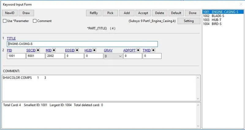
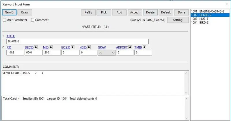
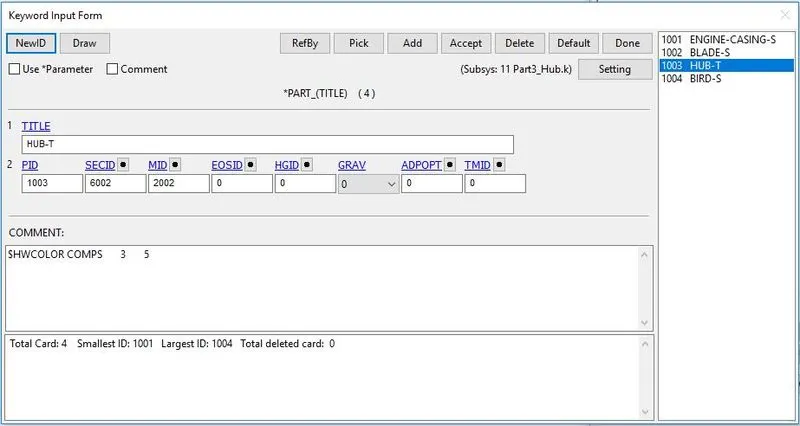
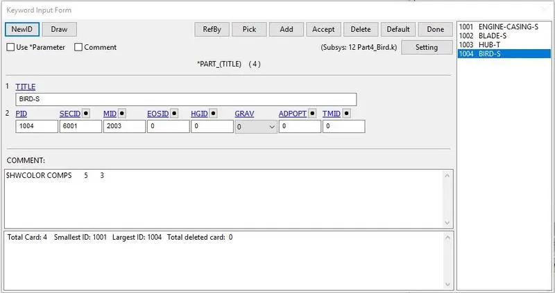
From the given file, all 4 parts are separated and saved individually. Here, the 4 parts are Engine Casing, Blade, Hub, and Bird respectively. Each part is assigned with section and material based on condition.

ENGINE_CASING

BLADES

HUB

BIRD

2. *Material_Definition:

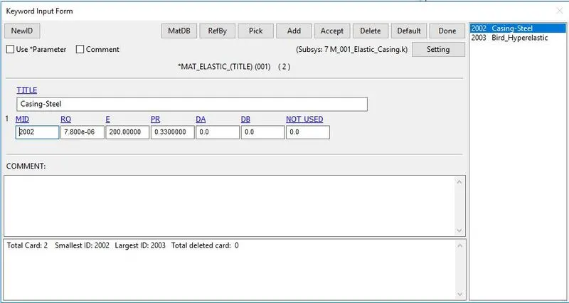
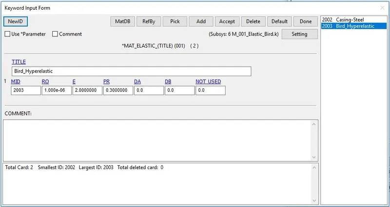
Here, the material used as M001_Elastic and M024_PIECEWISE_LINEAR_PLASTICITY. The elastic material is used for Casing, Hub, and Bird. M024 is used for Blades.

Elastic Material (M_001):

RO:=Mass density

E:=Young's modulus

PR:=Poisson's ratio

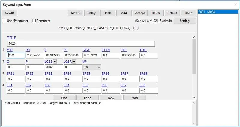
M024_PIECEWISE_LINEAR_PLASTICITY:

RO:=Mass density

E:=Young's modulus

PR:=Poisson's ratio

SIGY:=Yield stress

ETAN:=Tangent modulus, ignored if (LCSS.GT.0) is defined

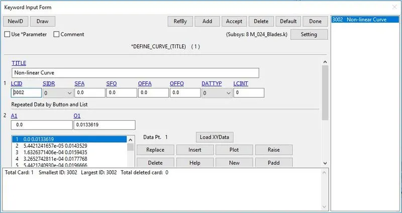
LCSS:=Load curve ID defining effective stress versus effective plastic strain.

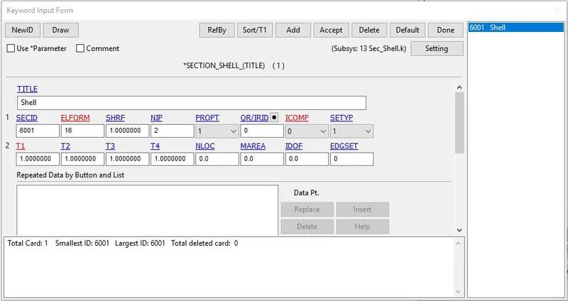
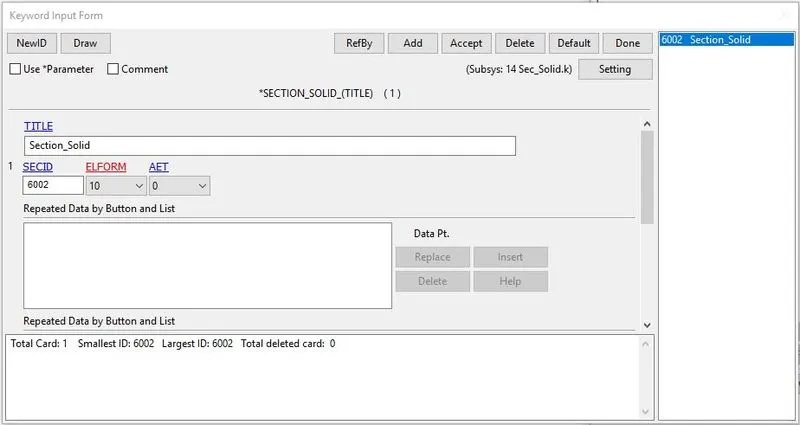
3. *Section_Definition:

ELFORM-16:=Fully integrated shell element (very fast)

SHRF:=Shear factor which scales the transverse shear stress (default =1.0)

NIP:=Number of through shell thickness integration points. Default is set to 2.

ELFORM-10:=1 point tetrahedron

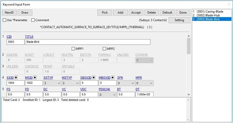
4. *Contact_Definition:

SSTYP:=Slave segment set or node set type (3).

MSTYP:=Master segment type (3).

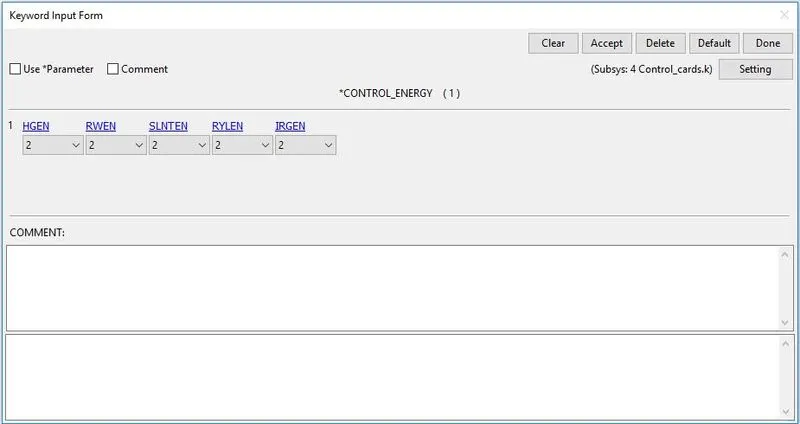
5. *Control_Definition:

HGEN:=hourglass energy is computed and included in the energy balance.

RWEN:=Stonewall energy dissipation is computed and included in the energy balance.

SLNTEN:=Sliding interface energy dissipation is computed and included in the energy balance.

RYLEN:=Rayleigh energy dissipation is computed and included in the energy balance.

ENDTIM:=Termination time is given as 5ms.

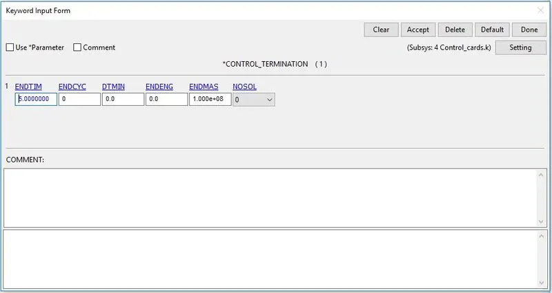
TSSFAC:=Scale factor for the computed time step. (Default =0.9. If high explosives are used, the default is lowered to 0.67).

DTINIT:=Initial time step size:0

DT2MS:=Time step size for mass scaled solutions (default set to 0.0).

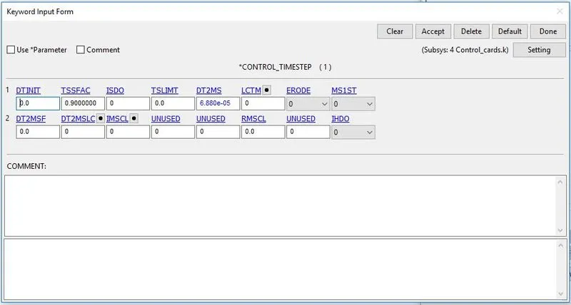
The units system is kg-mm-ms

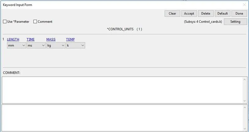
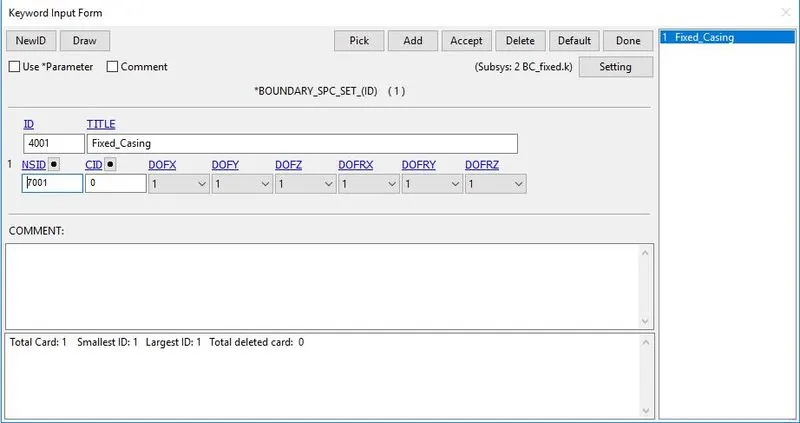
6. *Boundary_Condition: Here, The DOF is constrained in all directions.

7. *Database_Definition:

ELOUT:=Element Output Data

GLSTAT:=Global Statistics

MATSUM:=Material Energies

NODOUT:=Nodal Displacement/Velocity/Acceleration data

SLE:=Sliding Interface Energies

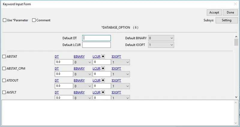
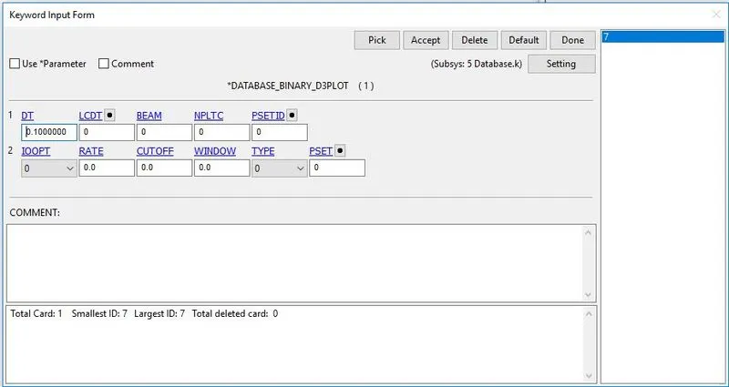
DT:=Time interval between outputs:0.1

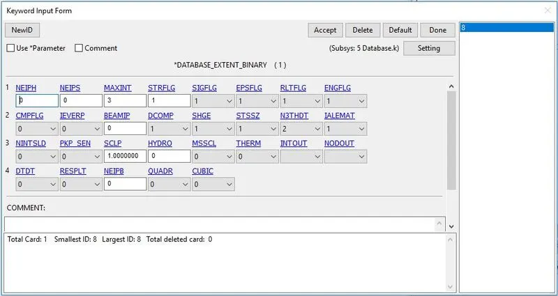
STRFLG-1:=Write plastic strain data to d3plot.
STRFLG-1:=Write thermal strain data to d3plot.

8. *Define_Curve:

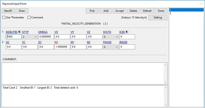
9. *Initial_Velocity_Generation:

VX:=Initial translational velocity in global x-direction.

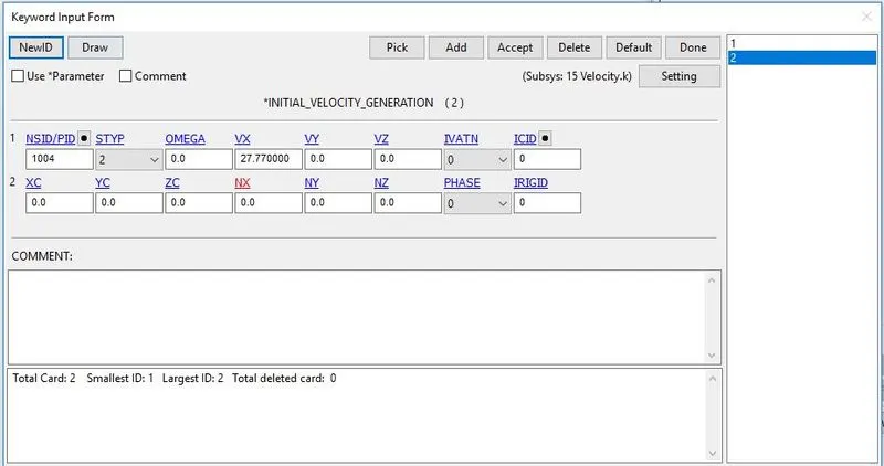
OMEGA:=Angular velocity about the rotational axis.

NX:=x-direction cosine.

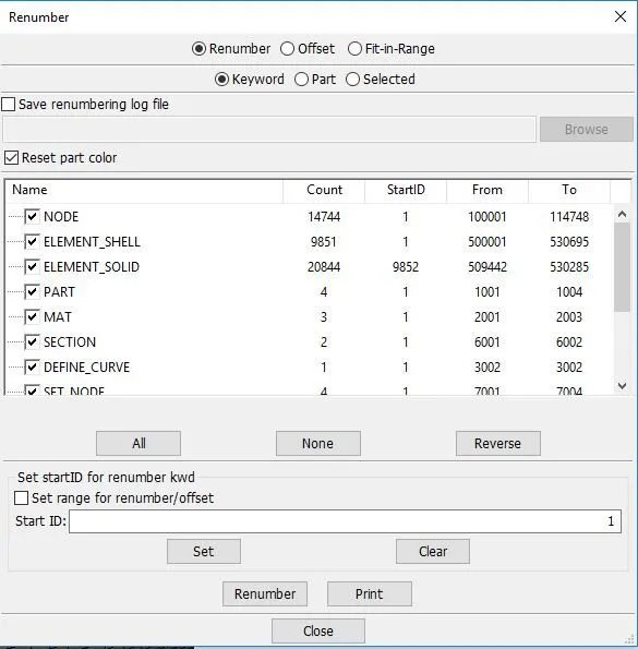
10. *Renumber_Definition:

11. *Keyword_Definition:

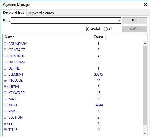
12. *Include_Definition: Once all the required cards as been created, then start to include the file in *INCLUDE card.

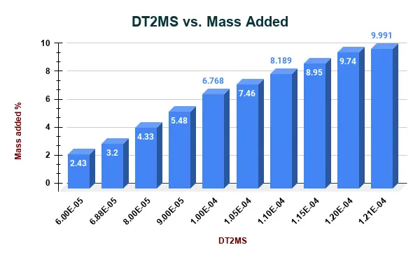
Mass_Scaling: TSSFAC: 0.9 & DT2MS: 6.88E-5

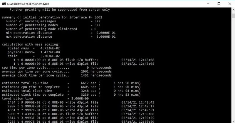
For these conditions, the mass added is 3.2 % and the estimated time is 54 mins.

TSSFAC: 0.9 & DT2MS: 6.00E-5

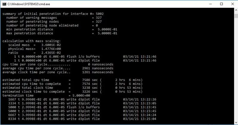
For these conditions, the mass added is 2.4 % and the estimated time is 53 mins.

TSSFAC: 0.9 & DT2MS: 8.00E-5

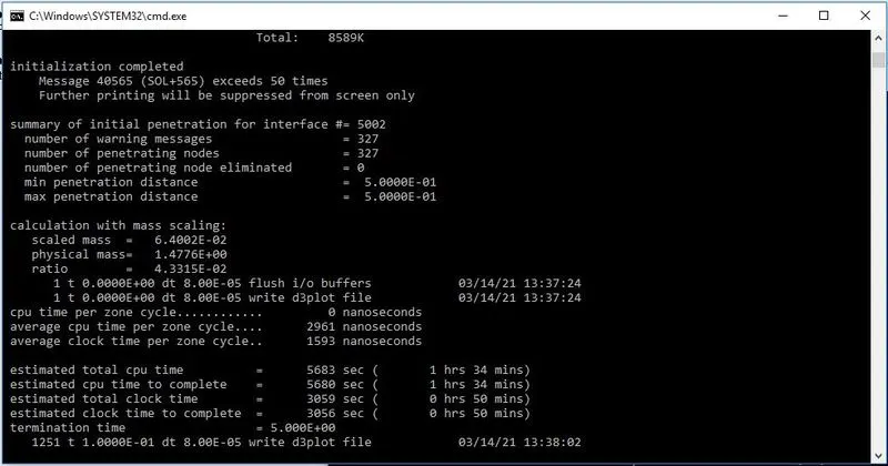
For these conditions, the mass added is 4.33 % and the estimated time is 50 mins.

TSSFAC: 0.9 & DT2MS: 9.00E-5

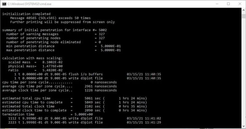
For these conditions, the mass added is 5.48 % and the estimated time is 35 mins.

TSSFAC: 0.9 & DT2MS: 1.00E-4

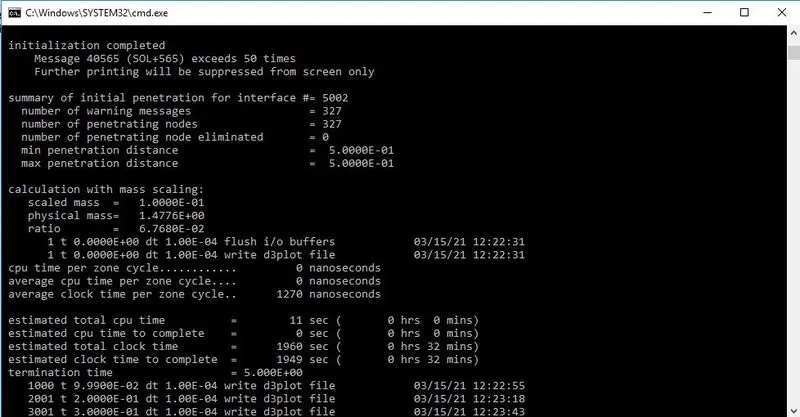
For these conditions, the mass added is 6.78 % and the estimated time is 32 mins.

TSSFAC: 0.9 & DT2MS: 1.05E-4

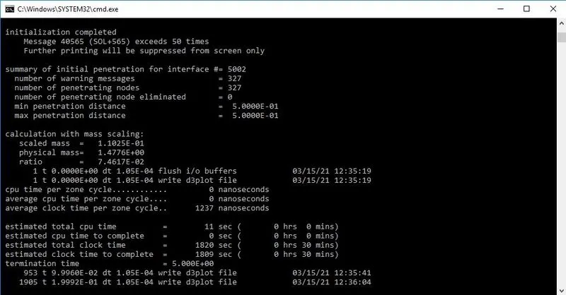
For these conditions, the mass added is 7.46 % and the estimated time is 30 mins.

TSSFAC: 0.9 & DT2MS: 1.10E-4

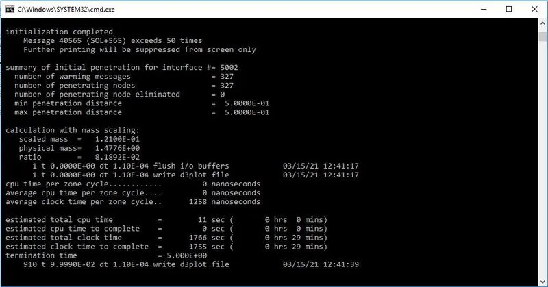
For these conditions, the mass added is 8.189 % and the estimated time is 29 mins.

TSSFAC: 0.9 & DT2MS: 1.15E-4

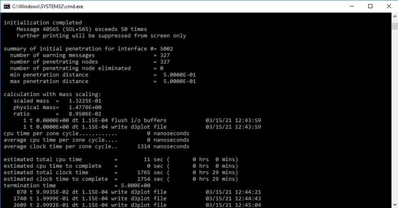
For these conditions, the mass added is 8.95 % and the estimated time is 29 mins.

TSSFAC: 0.9 & DT2MS: 1.20E-4

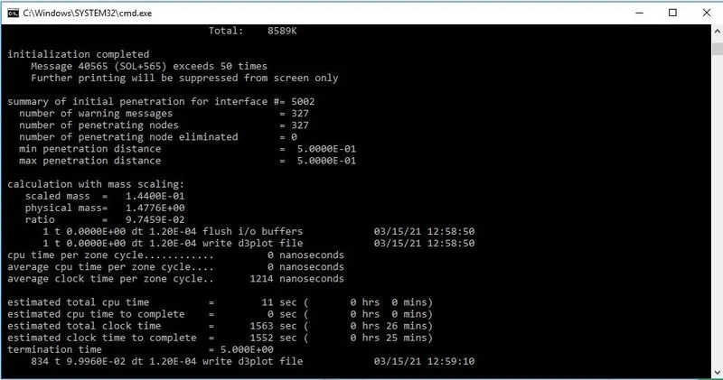
For these conditions, the mass added is 9.745 % and the estimated time is 26 mins.

TSSFAC: 0.9 & DT2MS: 1.21E-4

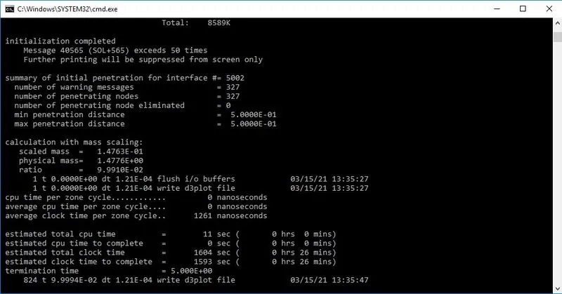
For these conditions, the mass added is 9.991 % and the estimated time is 26 mins.

RESULTS & DISCUSSION:

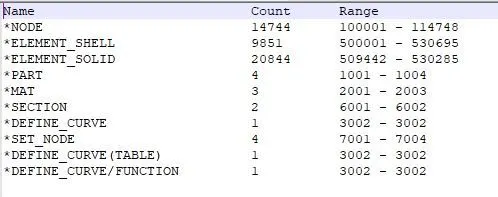
(i) Renumber of Nodes, Elements, Parts: The renumber is done by using a tool called Renumber under Model & Parts. The renumber is essential to identify the work easily and avoids the collaboration error.

(ii) Global Statics: In this Explicit Analysis, when the bird hits the blade at a velocity of 100kmph & at the time of 0.8 ms, the Internal energy increases and kinetic energy decreases due to the impact. There is no hourglass formation due to full integration ELFORM-16 is used.

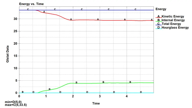
Hereafter the impact, there is still contact between the bird and blades which form sliding energy. In a real case, this will not happen very negligible.

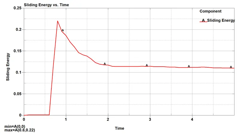
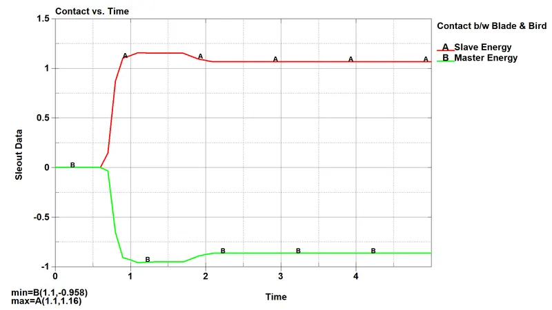
(iii) Sliding Interface Energies: Here, the bird is considered as the Slave part, and the blade is considered as the Master part. The Intersection energy between Blade and Bird is noticed here.

(iv) Time_History of Elements:

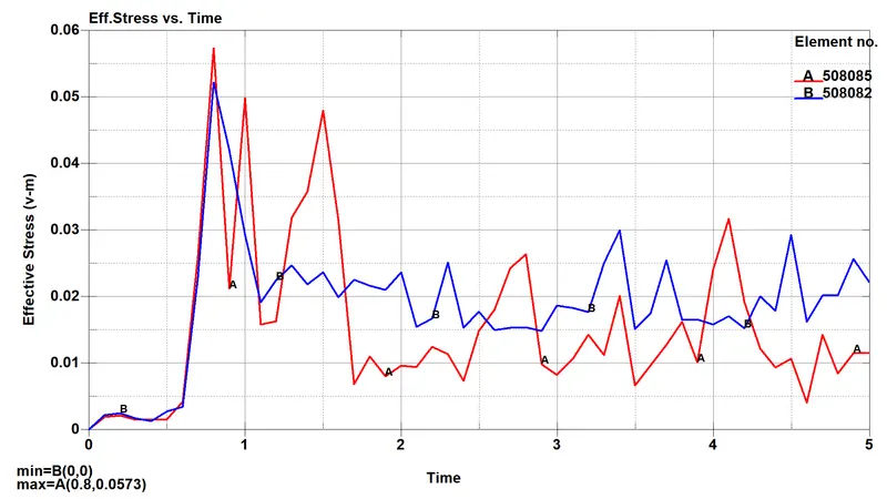
1. Effective Stress vs. Time: At the time of 0.8 ms, the bird hits the blade at a velocity of 100 kmph and the blade rotates at a velocity of 0.2 rad/s in a particular direction. The max stress developed is 0.058 Gpa in the blade.

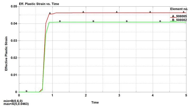
2. Effective Plastic Strain vs. Time: At the time of 0.8 ms, the bird hits the blade at a velocity of 100 kmph and the blade rotates at a velocity of 0.2 rad/s in a particular direction. The max plastic strain developed is 0.045 mm/mm in the blade.

(v) Contour Plots:

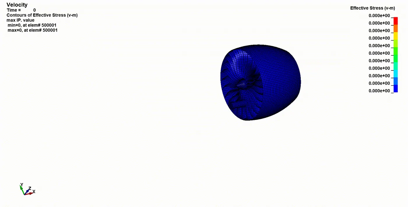
1. Effective Stress:

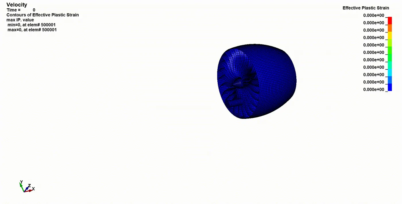
2. Effective Plastic Strain:

(vi) Mass Scaling Validation:

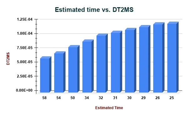
1. Estimated time vs. DT2MS: The value of DT2MS increases the time taken to complete the simulation reduces.

2. DT2MS vs. Mass Added: The value of DT2MS increases simultaneously the percentage of mass added also increases.

CONCLUSION:

1. All the subsystems are created and included in the Main_Include file.

2. From the literature review, assigned the material & section for different parts.

3. The simulation is run at 5ms and the animation is saved and attached here.

4. The Contour plots of Effective Stress & Effective Plastic Strain are obtained.

5. Mass Scaling is performed and obtained the results are maintained as 10%.

Drive_Link: https://drive.google.com/file/d/1gj3JvqACgZQ4HH4T4VfYAi7CdCVQ95IP/view?usp=sharing