Week - 8 Mass Scaling

Objective

To reduce the runtime of the model using the mass scaling technique and to achieve the following conditions shown below.

• The hard limit on mass scaling is 8% and stability should be completely intact.
• The DT and TSSFAC parameters should be optimized.
• Plot a histogram to compare the runtime with mass scaling trials.
• To run the same model using implicit solver with necessary changes and compare implicit and explicit runtime.

Introduction

Mass scaling refers to a technique whereby a non-physical mass is added to a structure to achieve a larger explicit timestep. One can selectively employ mass scaling by artificially increasing the material density of the parts you want to mass-scale. This manual form of mass scaling is done independently of the automatic mass scaling invoked within *CONTROL_TIMESTEP. When DT2MS is input as a negative value, mass is added only to those elements whose timestep would otherwise be less than |DT2MS|. By adding mass to these elements, their timestep becomes equal to |DT2MS|. An infinite number of combinations of TSSFAC and DT2MS will give the same product, i.e., timestep but the added mass will be different for each of those combinations. The trend is that the bigger |DT2MS| (and the smaller TSSFAC while TSSFAC*|DT2MS|=const), the greater the added mass. In return, stability may improve as TSSFAC is reduced (just as in non-mass-scaled solutions). If stability is a problem with the default TSSFAC of 0.9, try 0.8 or 0.7. If you reduce TSSFAC, you can increase |DT2MS| proportionally so that their product, and hence timestep, is unchanged.

A mass scaling operation has been performed to reduce the runtime of a model and ensure the model's stability. The hard limit on mass scaling taken up to 8% and ensuring the stability of the model completely during the process. Here a trial and error method has been followed and when the mass scaling objective has been reached, a histogram has been plotted to compare the run time with the mass scaling trails. Also, the same model has been run used implicit solver with necessary changes and compared the implicit and explicit runtime.

Procedure

• The given (.k) file of the model has been opened on ls-prepost.

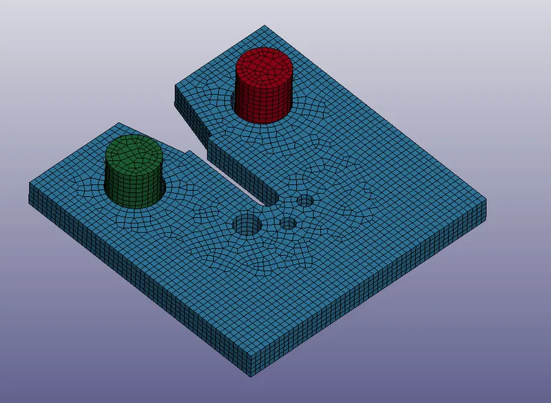
• The model has been checked for any errors and it's been saved and run using ls-program manager.

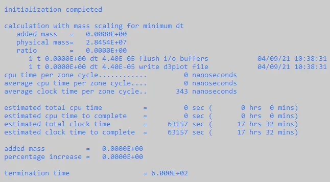
• Here the model was run without any mass scaling and the total time estimated is around 17hrs 32mint.
• The model was again opened in ls-prepost and then checked the*CONTROL_TIMESTEP card. The default values for TSSFAC and DT2MS were given 0.9 and -3.5e-05 respectively.
• Now DT2MS value has been incremented by a unit one keeping TSSFAC to a constant value (0.9).
• A trial and error method was followed and the process has been continued until it shows a percentage increase of around 8%.

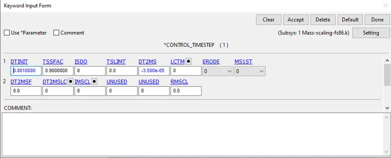
TSSFAC= 0.9 and DT2MS= -4.5e-05

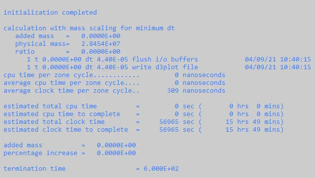
• Here a decrease in the estimated run time has been obtained (15hrs 49min) and there is no added mass and percentage increase.

TSSFAC= 0.9 and DT2MS= -5.5e-05

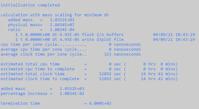
• Now the mass gets added and the percentage increase was found to be 0.010034, which is well beyond the required value. The process has been further continued till we get a percentage increase of around 8%.
• The results for the remaining timestep have been tabulated shown below.

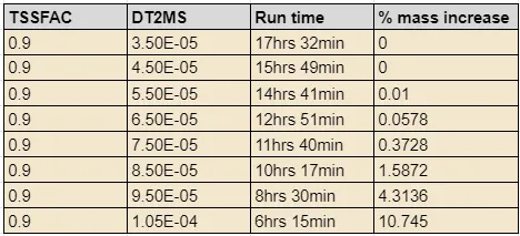
• The table shows that the run time gets reduced when the DT2MS value was incremented and when it reached 1.05e-04 the percentage increase was above the required value and the percentage mass increase shown for the lower value is 4.3136 and for the upper value it's 10.745 Also, the total runtime was found to be 6hrs 15min.
• The same process was again carried out by changing the TSFAC value to 0.8 and incrementing the DT2MS value.

TSSFAC= 0.8 and DT2MS= -4.5e-05

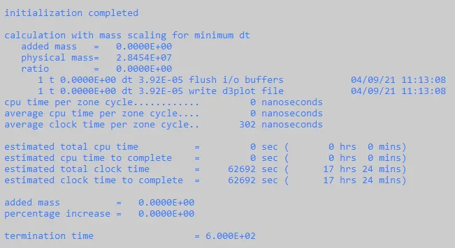
• The estimated time for this case with TSSFAC= 0.8 and DT2MS=-4.5e-05 was found to 17hrs 24mins which is more when compared to TSSFAC= 0.9. Here also there no no added mass and percentage increase.

Timestep | TSSFAC= 0.8 and DT2MS= -5.5e-05 |

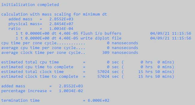
• Like that of the above case with TSSFAC with 0.9, here also the mass gets added and shows a percentage increase for the corresponding DT2MS value. The process has been further continued till we get a percentage increase of around 8%.
• The results for the remaining timestep have been tabulated shown below.

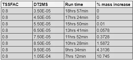
• The table shows that the run time gets reduced when the DT2MS value was incremented and when it reached 1.05e-04 the percentage increase was above the required value and the total runtime of 7hrs 12min was shown which is more than that of TSSFAC with a value of 0.9.
• Now the simulation was again performed using the TSSFAC=0.9 by splitting the DT2MS value and by incrementing this DT2MS value the iteration process has been carried out until it shows an added mass percent up to 8.

Implicit method

• An implicit analysis was also done to the current model for the study purpose.
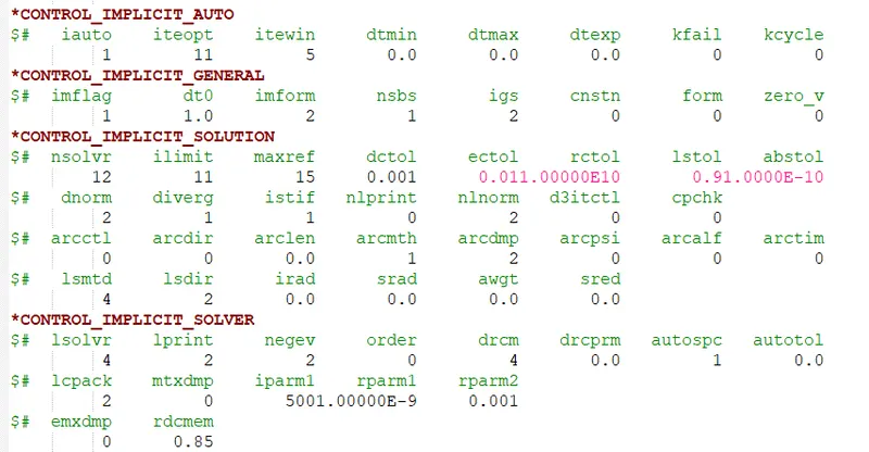
• The following cards were activated from the keyword manager and assigned with the required values.
• *CONTROL_IMPLICIT_GENERAL: The keyword makes sure that the analysis will start in an implicit manner since the default analysis mode for ls Dyna is explicit. Here the IMFLAG is set to 1 to activate the implicit analysis.
• *CONTROL_IMPLICIT_AUTO: Used to change the time step for the given problem. In implicit the time step can be changed since its unconditionally stable but in explicit analysis, the time step is the condition beyond a certain value. Here IAUTO is kept as one.
• *CONTROL_IMPLICIT_SOLUTION: Used to specify whether the analysis should be linear or non-linear static. In general for non-linear analysis, the default solution method (NSOLVR=12) is perfectly adequate. If contact is specified in the model then the analysis is non-linear regardless of the loading or material properties.
• *CONTROL_IMPLICIT_SOLVER: Used to specify the linear equation solver used to perform the stiffness matrix inversion(LSOLVR). In general, the default solver (NSOLVR=4) is perfectly adequate for SMP.

Results and discussions

• Performed simulations, One without mass scaling and one with mass scaling for the given model by a trial and error method. The hard limit on mass scaling was set as 8% and ensured the stability of the model. The simulation was also done using an implicit solver in order to study the behavior and for the comparison of results.
• The estimated total time is not the actual time to finish the simulation, it may take lesser than the estimated time. It differs from systems to systems depending upon the processor and system configuration.
• A histogram was plotted to compare the run time for various TSSFAC and DT2MS values, which is shown below.

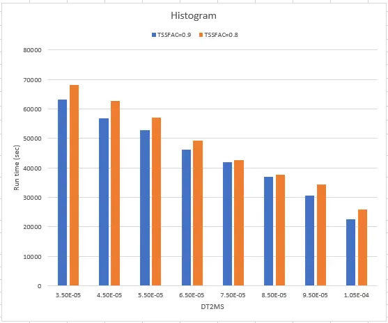
• From the plot, it's clear that the run time gets minimum when the simulation was performed with TSSFAC=0.9 when compared to TSSFAC=0.8. So TSSFAC=0.9 was taken as the optimum value.
• The minimum run time using mass scaling for this simulation was found to be 6hrs 15min with a TSSFAC value of 0.9 and DT2MS=0.000105. But the percentage increase in mass was found to be 10.745%, Which was more than the target value ie, 8%. Therefore the simulation was again performed by splitting the regions of DT2MS further between 0.000095 and 0.000105 and thereby incrementing the values again.
• The values are tabulated as shown below.

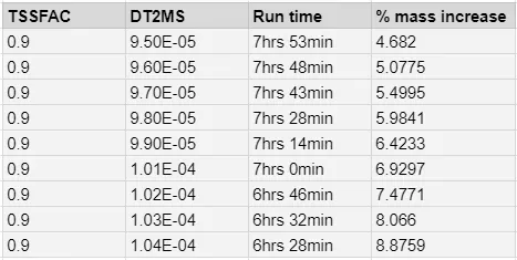
• So from the table, We get the required mass scaling with a 7.4771% increase at TSSFAC=0.9 and DT2MS=0.000102. Further incrementing the DT2MS will increase the percentage mass above 8%, which is not acceptable.

Results from implicit analysis

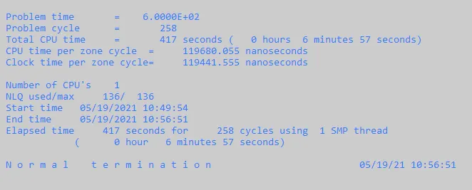
• The elapsed time took to slove using the implicit method was around 417 seconds which was very less but for accuracy, the time step has to be well considered here.
• The total run time for the simulation using an implicit solver cannot be predicted at the start of the simulation as it considers global equilibrium and requires a series of trial solutions (iterations) to establish equilibrium within a certain tolerance. Thus we cannot compare the explicit analysis with implicit analysis.

Conclusion

• The mass scaling for the given model has been performed as per the objective and compared the results.
• Its been found that when a mass scaling factor is applied, the mass of the elements with a time increment below a certain value is scaled. By adding a mass to these critical elements, the calculation time is decreased.

............................................................................................................................................................................................................

File: https://drive.google.com/drive/folders/11pud9Ki2fXtEMxZqg5z2aJUyhqTAgewN?usp=sharing