Week-6 Calculate the Stretch Ratio by comparing the ELFORM (-2,-1,1,2) with Ogden_Material Model.

Objective

• To create a solid block of given dimension with 10 elements for each directions to understand the uniaxial behaviour and to compare the results for the simulation using ELFORM = 1, 2, -1, -2.

Deliverables:

• An excel sheet with proper conversion and calculation of Stress/Strain and the Stretch Ratio for all the ELFORM.
• A proper image of the plot comparison of various ELFORMS against the Uniaxial Plot given in the challenge.

Introduction

• Explicit and implicit methods are mainly used to solve dynamic events with a governing equation `[M]{x''}+[C]{x'}+[K]{x}={f}`. Implicit and Explicit analysis differ in the approach to time incrementation. In Implicit analysis each time increment has to converge, but you can set pretty long time increments as this method is used for solving static and quasi-static problems. Explicit on the other hand doesn’t have to converge each increment, but for the solution to be accurate time increments must be super small. This equation can also be used to solve static problems by considering the mass and damping matrix as null matrix. But solving this algorithm with this method are expensive as compared to direct static schemes.
• Here the simulation for the tensile problem was performed using ogden material which is hyper-elastic and a non-linear material and thereby solving it through implicit method as the rate of displacement is very low. An explicit method can also be used to solve the problem but it will take more time for the solve it explicitly.
• In Ls-dyna there are different element formulation (Elform) available which is based on integration points and is being used according to the required criteria. A lesser number of integration points reults in lower accuracy of the results but requires only low computational time and more number of integration points results in higher accuracy but takes more computational time.
• The current simulation is performed using different elform and thereby comparing there results.
• The unit system followed for the simulation are in gm,mm,ms.

Procedure

Creating a solid cube.

• The file (Ogden_material.k) has been opened in Ls-prepost which contain the given problem statements.
• A solid cube of 10mmx10mmx10mm dimension with 10 elements for each direction was created using "Element and mesh> Shape mesher.

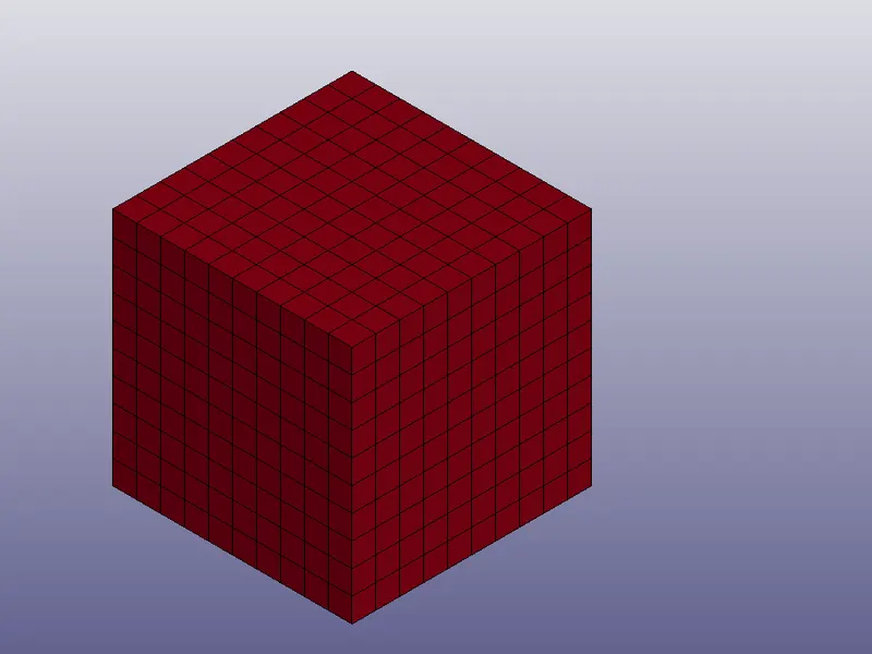
Assigning material and section to the part.

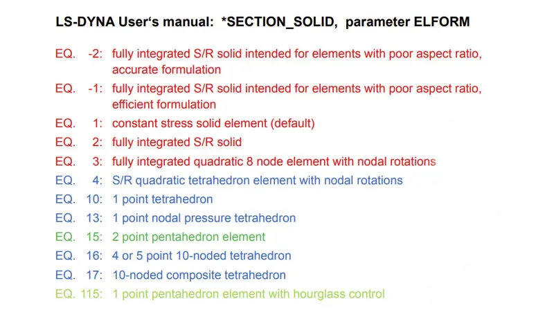
• A *SECTION_SOLID card with Elform=1 initially was created for the cube using "Keyword manager>section>soild.
• Three more simulations were carried out further using Elform of -1, 2, -2 respectively.

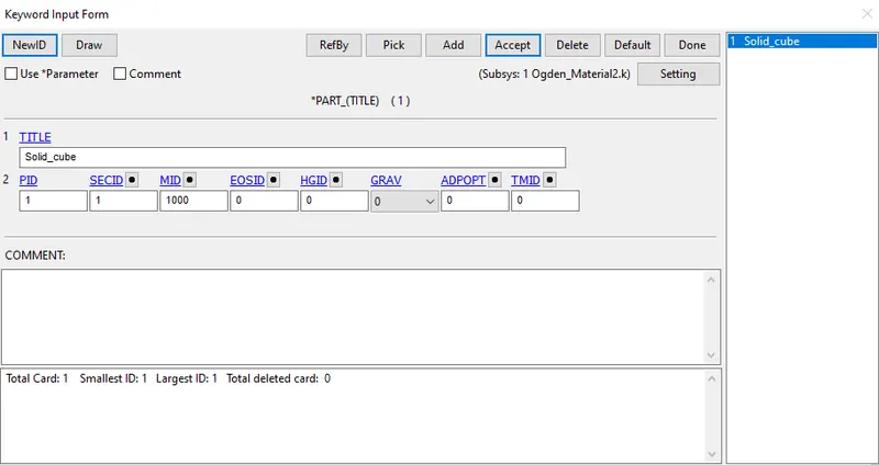
• The given file already contained the required material card which is hyper-elestic one with the card name *OGDEN_RUBBER and no further changes has been done.
• The section card and material card were then assigned to the part id.

Boundary conditions.

• Since we are performing tensile test, the part will elongate with respective to the load. Here the two boundary conditions like SPC and Priscribed motion set have been used.
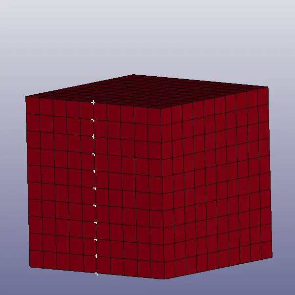
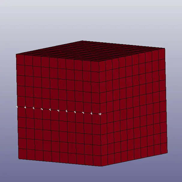
• A SPC boundary condition has been given as shown below where the translational motion in y and z direction were allowed.

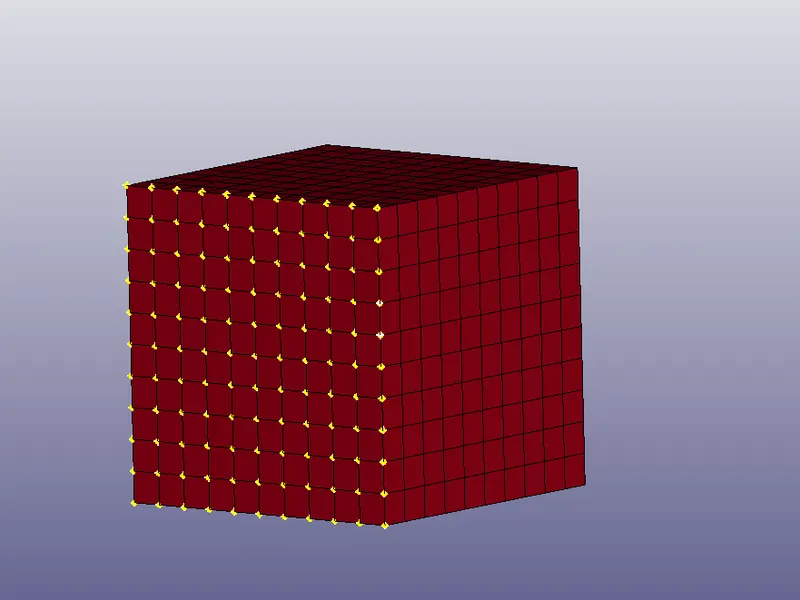
• Two more SPC were created which will constrain the nodes along translational y and other translational z direction respectively as shown below.

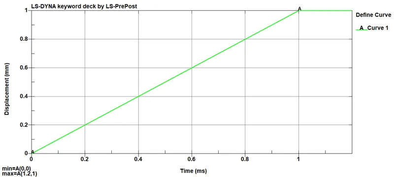
• Before giving the displacement through *BOUNDARY_PRISCRIBED_MOTION_SET card, a load curve has to be defined so the displacement can be applied uniformly.
• Load curve can be created using " Keyword manager>Define>Curve.
• The graph has to plotted upto stretch ratio of 5. Therefore the minimum displacement needed is found to 40mm and the displacement was defined upto 45mm.
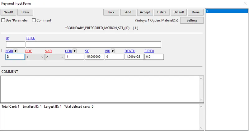
• The scale factor can be assigned in the boundary card.
• Whenever creating a load curve its a recomendable to extend the curve beyond the termination time.

• A node set was also created as shown below.

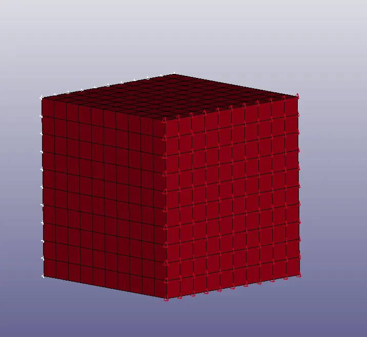
• Finally the cuve id and other parameter values like VAD and DOF (translation along x axis) were assigned to the *PRESCRIBED_MOTION_CARD from the keyword manager.

Control cards for implicit analysis.

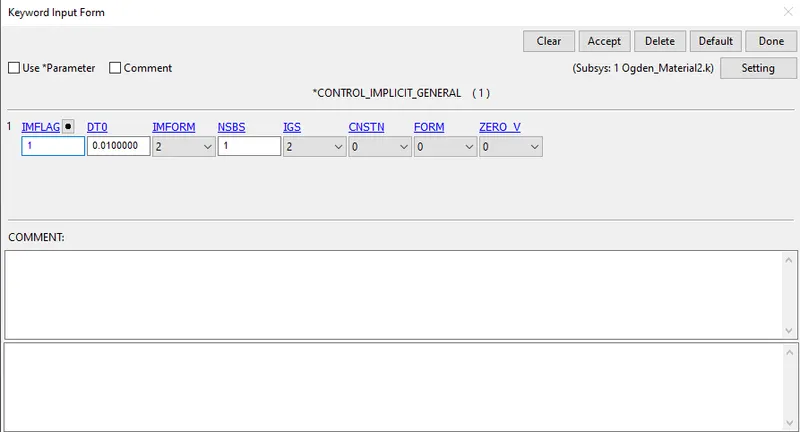
• *CONTROL_IMPLICIT_GENERAL: The keyword make sure that the analysis will start in an implicit manner since the default analysis mode for ls dyna is explicit. Here the IMFLAG is set to 1 to activate the implicit analysis.

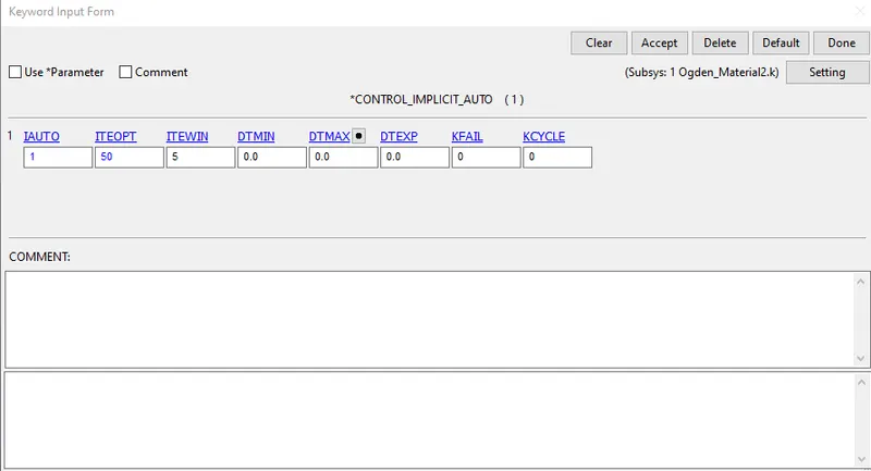
• *CONTROL_IMPLICIT_AUTO: Used to change the time step for the given problem. In implicit the time step can be changed since its unconditionally stable but in explicit analysis the time step is the condition beyond a certain value.

• *CONTROL_TERMINATION_CARD from keyword manager is used to define the simulation time using ENDTIME otpion.

Database.

• The oputput data needed for the analysis is generated using *DATABASE card.
• DATABASE_BINARY_D3PLOT under keyword manager ensures d3plot files are written in which it stores the stress strain contours of the deformed system.
• ASCII under keyword manager can generate different output such as force generated in a contact, total energy, material engery etc. Here output for GLSTAT, NODOUT have been requested.
• DT (Time intervel between the output) is an essential parameter which basically denotes the time intervel after which the state of solution need to be written and the value is kept as 0.01 for this analysis.
• *DATABASE_EXTENT_BINARY card was provided by specifying STRFLG (1) which write strain tensor data to d3plot and elout.

Model check up and running the simulation.

• The model is checked for any errors and if any error occurs it should be corrected further.
• The .k file is been saved and runned using LS-DYNA manager.
• A memory of 10000000 is assigned to the setup to run the analysis in core memory.

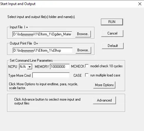
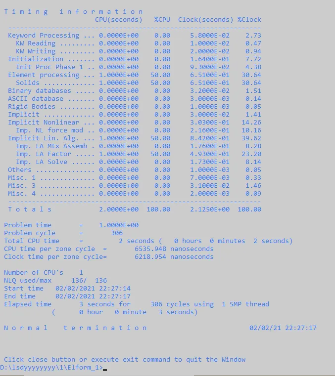
• If Normal termination is showed after running the file, its then ready to do post processing.

Calculation

• The stress-strain data obtained from Ls-dyna during the analysis was given for true stress and true strain. Therefor the these data have been converted to engineering stress and strain data also the engineering strain can be converted to stress ratio using the formula given below.
• `epsilon_(true)=ln(1+epsilon_(eng))`
• `sigma_(true)=sigma_(eng)(1+epsilon_(eng))`
• `lambda=1+epsilon_(eng)`
• `epsilon_(true)` : True strain
• `epsilon_(eng)` : Engineering strain
• `sigma_(true)` : True stress
• `sigma_(eng)` : Engineering stress
• `lambda` : Stretch ratio

Results

• Solid block of given dimension with 10 elements for each directions were created and performed a uniaxial tensile test to find out the its behaviour under different ELFORM and the results of the simulation has been compared from the plot upto a stretch ratio of 5.

Animation

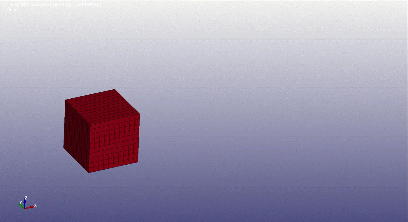
Stress contour

Strain contour

• Since the elongation of the cube is only in x-direction it shows a uni-axial behaviour. The values for the x stress and lower ipt x-strain where taken using history>elements, which gives the true stress-strain data and its been converted to engineering data to plot the curve.
• The simulation was performed with ELFORM 1,-1,2,-2 and found out the stress and stain corresponding to it along with stretch ratio up to 5 and compared the results.
• Plots of engineering stress vs stretch ratio with different element formulation are shown below.

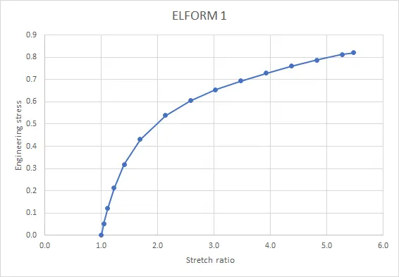
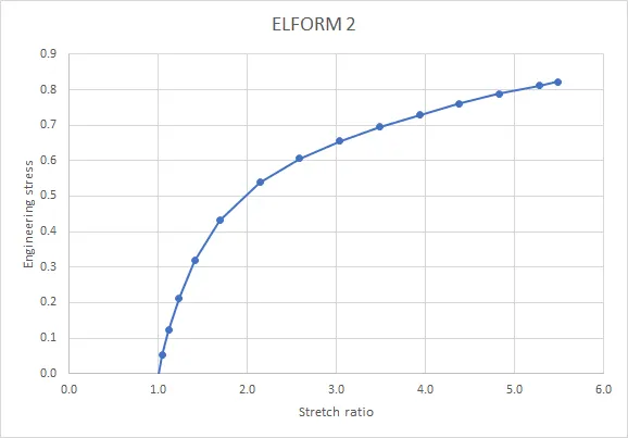
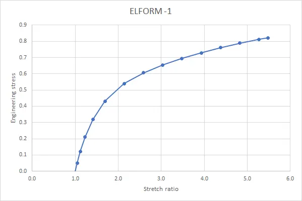
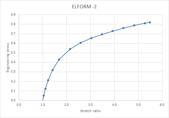
• From the above plots its observed that various ELFORM shows similar type of behaviour. There is only a small variation in computational time for various ELFORM. Its due to the simplicity of the model and if the model was complex and showed large deformations, we would be able to observe the difference.

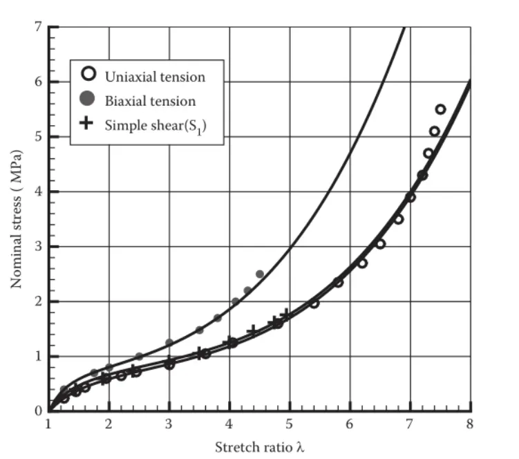
• The actual stress vs stretch ratio for the Ogden model is shown above. It can observed that the stress induced at stretch ratio of 5 is approximately equals to 1.8MPa. When compared with the simulation performed with various ELFORM shown above shows stress value of around 0.82 at a stretch ratio of 5, which is very less when compared to the original one. Its again due to the simplicity of the model or due to variation in rate of loading etc.

Conclusion

• A uni-axial tensile test was performed as per the objective and requested output were obtained. The simulation was carried out using implicit method as the rate of displacement is very low. An explicit method can also be used to solve the problem but it will take more time for the solve it explicitly. The results of the true stress-strain data were then converted to engineering data and plotted a curve between engineering stress and stretch ratio. The proces were carried out for various ELFORM and then compared the result.
• Some of the ELFORM of Hexahedral elements are discussed below.

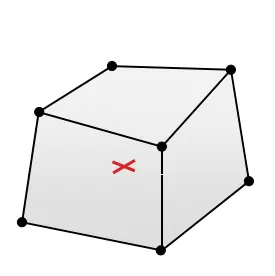
ELFORM 1

• Under integrated constant stress.
• Efficient and accurate.
• Even works for severe deformation.
• Need hourglass stabilisation : Choice of hourglass formulation and value remains and issue.

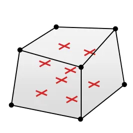
ELFORM 2

• Selective reduced integrated brick element (Volume locking alleviated).
• No hourglass stabilisation needed.
• Slower than ELFORM=1.
• Too stiff in many situations, especially poor aspect ratio (Shear locking).
• More stable in large deformation applications.

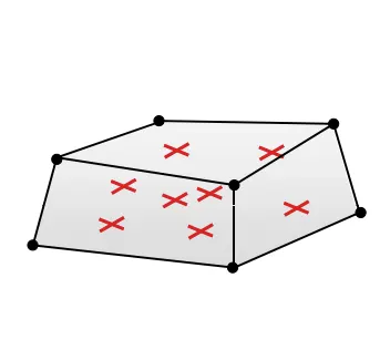
ELFORM -1

• Identical with type 2 but accounted for poor aspect ratio in order to reduce shear locking.
• Efficient formulation.
• Sometimes hourglass tendencies.

ELFORM -2

• Identical with type 2 but accounted for poor aspect ratio in order to reduce shear locking.
• Accurate formulation.
• Higher computational cost than type -1.

.............................................................................................................................................................................................................

File: https://drive.google.com/drive/folders/1hpxf7jaUPrAF-41u3Wwht3fvR-0AA0D8?usp=sharing