Week - 10 Hyperelastic Material Models

Objective

To calculate the Mooney Rivlin and Ogden material constants and compare both using stress-strain data from a Dogbone specimen tensile test with 100 percent strain.

Introduction

Hyperelastic materials are the special class of materials that respond elastically even when they are subjected to large deformations. They show both a nonlinear material behavior as well as large shape changes. They are characterized by:

1. Can undergo large elastic deformations in order of 100 to 700% which are fully recoverable, i.e., the initial shape is recovered when the load is removed.
2. Are nearly incompressible, which means that they change can their shape but overall volume remains almost constant.
3. Show a highly nonlinear stress-strain relation.
4. The material softens and then becomes stiffer again when applied to tension whereas, under compression, they have a quite stiff response.

Many polymers show hyperelastic behavior, such as elastomers, rubbers, and other similar soft flexible materials.

Hyperelastic materials are mostly used in applications where high flexibility, in the long run, is required, under the presence of high loads. Some typical examples of their use are elastomeric pads in bridges, rail pads, car door seals, car tires, and fluid seals.

Procedure

• The data for the given engineering stress-strain values were arranged and plotted a curve in an excel sheet.

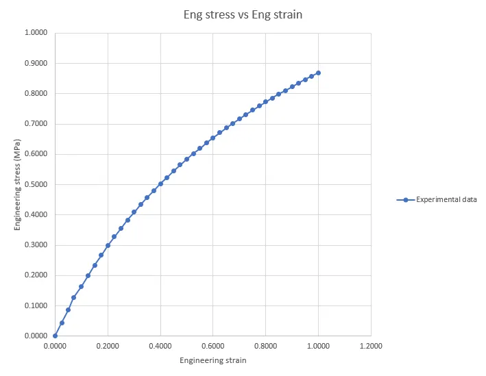
• Now the .k file of the given model was opened in the Ls-Pre post.

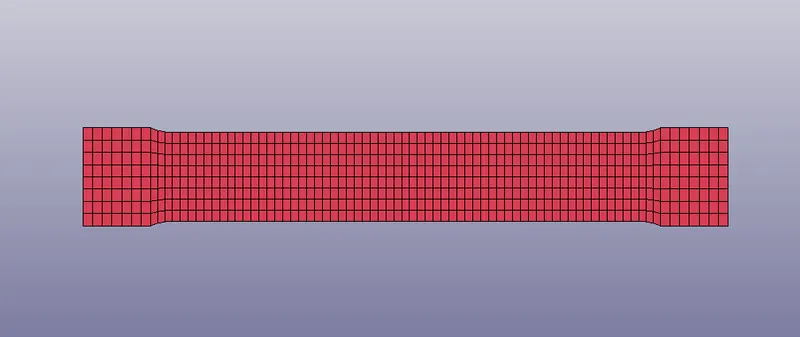
Defining material and section to the part

• *MAT_HYPERELASTIC_RUBBER card was used while modeling the first specimen *MAT_ODGEN_RUBBER was used for the second one.
• Other parameters such as density, Poisson's ratio, N (Number of constants to solve for) LCID were also assigned. The LCID was assigned with the data taken from the excel sheet. It can easily be assigned with the help of notepad++.

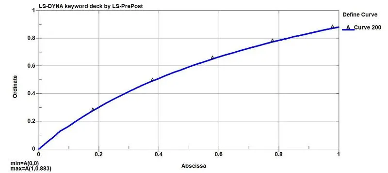
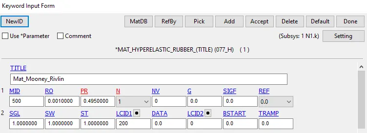
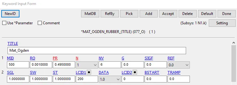
• Initially, the value for N in the material card was kept as one and it been changed to two and three after each run and found out the constants needed for the final run.
• From the Ls-dyna manual, it's said that Load curve ID giving the force versus actual change in the gauge length. If SGL, SW, and ST are set to unity (1.0), then curveLCID1 is also engineering stress versus engineering strain. The curve should have both negative (compressive) and positive (tensile) values.

Boundary conditions

• The displacement was given to the end nodes using *BOUNDARY_PRISCRIBED_MOTION_SET. The value for the displacement was calculated as follows.

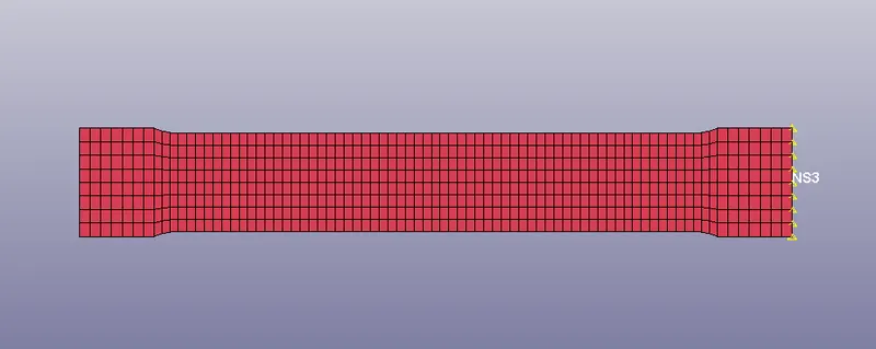
• To calculate the displacement for the boundary condition, we know 100 percent strain equals a stretch ratio of value 2.

`lambda=1+epsilon_e`

`epsilon_(true)=ln(1+epsilon_e) implies epsilon_(true)=ln(2)`

Strain=(Change in lenght)/original lenght

Therefore, Change in lenght or displacement = `ln(2)*145=100`

`lambda`=Stretch ratio

`epsilon_e`=Engineering strain

`epsilon_(true)`=True strain

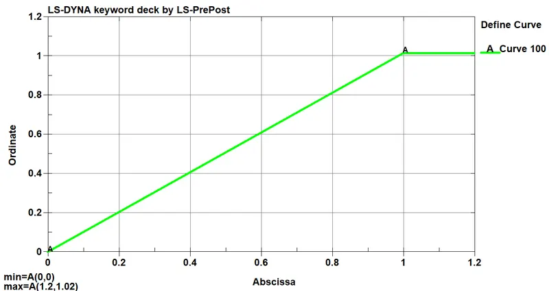
• This value has been assigned to the load curve scale factor also a load curve has been created to define the displacement.

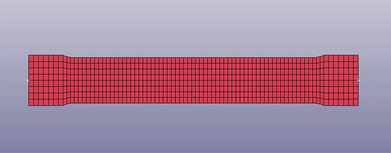
• The nodes at the other end of the model are fixed in all DOF except at translation along the y-axis using single point constraint(SPC).

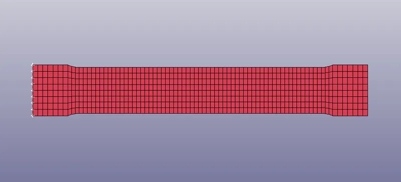
• Also, two more nodes are constrained only in the y-direction as shown in the figure below to describe the actual behavior of the model.

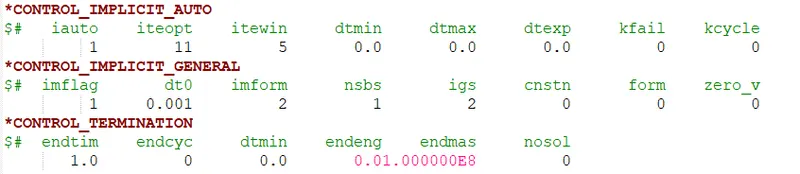
Control cards for implicit analysis.

• *CONTROL_IMPLICIT_GENERAL: The keyword makes sure that the analysis will start in an implicit manner since the default analysis mode for ls dyna is explicit. Here the IMFLAG is set to 1 to activate the implicit analysis.
• *CONTROL_IMPLICIT_AUTO: Used to change the time step for the given problem. In implicit the time step can be changed since its unconditionally stable but in explicit analysis, the time step is the condition beyond a certain value. Here IAUTO value was kept as one.

• Apart from this other cards such as *DATA_BASE_EXTENT_BINARY, *DATABASE_ASCII, and BINARY_D3PLOT were created to get the required outputs.
• The end time was defined as one using the *CONTROL_TERMINATION card.

Model check-up and running the simulation.

• The model is checked for any errors and if any error occurs it should be corrected further.
• The .k file is been saved and ran using LS-DYNA manager.
• If Normal termination is showed after running the file, it's then ready to do the post-processing.

Results

For Mooney Rivlin constant(Hyperelastic rubber)

• The simulation was initially performed by changing the N values from the material card in order to find out the Mooney-Rivlin constant.
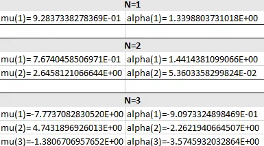
• The values for the constants can be seen in the d3hsp file. The value for the constants is shown below.

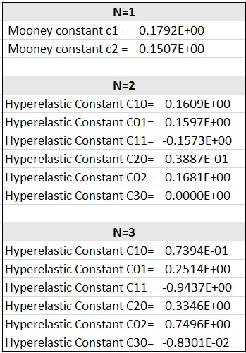
• Data for stress-strain values are also collected from the d3hsp file and it been converted to engineering stress-strain to compare with the experimental data.
• A graph was plotted to compare the experimental data with the values that got from the Mooney-Rivlin constants Which are shown below.

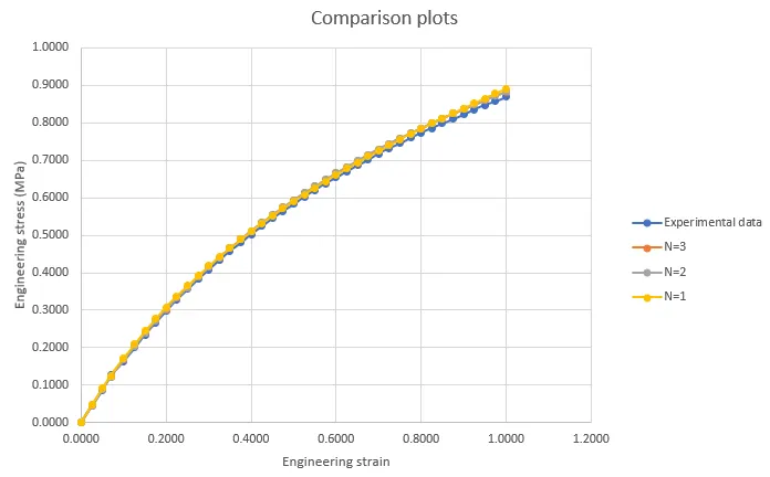
• From the graph, it can be observed that the almost the three curve fits with the experimental data. The constant N=3 was chosen because it's comparatively in range with the experimental data curve.
• Now the material card can be modified using the Mooney-Rivlin constant corresponds to N=3 as shown below. Finally, the model can be again run in the Ls-program manager to get the required output.
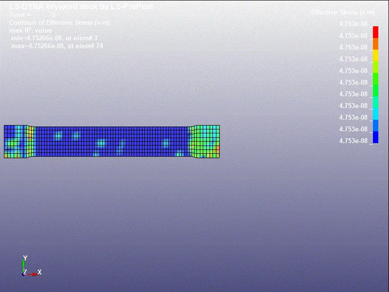
• The below animation shows the effective stress for the specimen that was modeled with an updated material card.

For Ogden material constants

• The simulation was initially performed by changing the N values from the material card in order to find out the Ogden material constant.
• The values for the constants can be seen in the d3hsp file. The value for the constants is shown below.

• A graph was plotted to compare the experimental data with the values that got from the Ogden material constants Which are shown below.

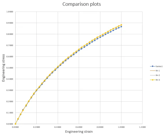
• From the graph, it can be observed that the almost the three curve fits with the experimental data(blue curve). The constant N=3 was chosen because it's comparatively in range with the experimental data curve.
• Now the material card can be modified using the Ogden material constant corresponds to N=3 as shown below. Finally, the model can be again run in the Ls-program manager to get the required output.
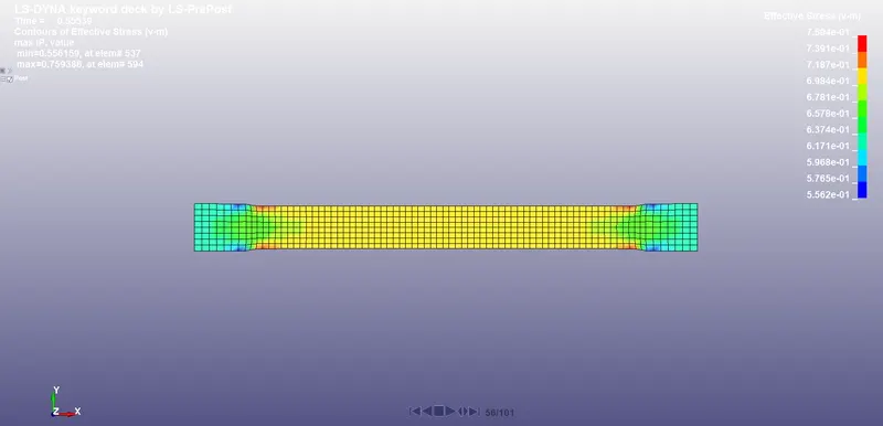
• The below plot shows the effective stress for the specimen that was modeled with an updated material card.

Conclusion

• From the given material data, calculations were done using the Mooney Rivlin and Ogden material constants and compared both using stress-strain data from a Dogbone specimen tensile test with 100 percent strain. Here the test was done by changing the N values in the material card to find out the best fit to model the material. For the two cases, N3 was chosen since it's very closer to the given data.

............................................................................................................................................................................................................

File: https://drive.google.com/drive/folders/1uR1h-RdJSjjK5yMqWVKlJbYhK8DfvcH0?usp=sharing