EXPLICIT AND IMPLICIT ANALYSIS_CALCULATIONS.

OBJECTIVE:

To solve the given equation using implict and explit methods with a residual tolerance of 0.01.

Equation: `F(u)=u^3+9u^2+4u`

F- Force in the bar, u- Displacement in the bar.

EXPLICIT/IMPLICIT METHOD

Explicit and implicit methods are mainly used to solve dynamic events with a governing equation `[M]{x''}+[C]{x'}+[K]{x}={f}`. Implicit and Explicit analysis differ in the approach to time incrementation. In Implicit analysis each time increment has to converge, but you can set pretty long time increments. Explicit on the other hand doesn’t have to converge each increment, but for the solution to be accurate time increments must be super small. This equation can also be used to solve static problems by considering the mass and damping matrix as null matrix. But solving this algorithm with this method are expensive as compared to direct static schemes.

IMPLICIT METHOD

• In implicit scheme the unknown factor (`x`) is found out by inversion of stiffness matrix.
• For each increment of load the stiffness matrix is updated (If needed mass matrix is also updated). Then an incremental load will be defined and when the governing equation is defined for the next increment , Newton Raphson method is used to solve the problem using iterative method.
• Thus this method gives more accurate results when compared to explicit method.
• This method is prefferable when the strain rates are minimim.
• Implicit schemes are time consuming for large models and are unconditionally stable.
• Here there is no mathematical time limit for the solution and requires much more storage space in computer.
• Applications: Good choice for structure dynamics problems for which load rate is slow. Eg: Low frequency response, vibration, oscillation etc.

EXPLICIT METHOD

• In explicit scheme the unknown factor (`x`) is found out by inversion of mass matrix.
• Here also the matrix are updated and an incremental load is defined but like that of implicit method there is no need of itration process, direct solution is possible.
• Less accurate when compared to implicit scheme.
• This method is prefferable when the strain rates are high and can solve extremely discontinuous events or process.
• Time taken by the explicit analysis depends on wave propagation speed and characteristic lenght of the element and can predicit the time taken for the anlslysis.
• Applications: For wave propagation types of problems such as crash analysis, drop, blast etc.

CALCULATION:

Using explicit method:

• Equation: `F(u)=u^3+9u^2+4u`
  
• If the nonlinear force versus displacement relationship is not known, but the stiffness is known, it is possible to construct the graph of force versus displacement numerically.
• One method is to use an incremental explicit load control scheme. Here three equal load increments (or steps) of `DeltaF` unit each are used to load the tension bar.
• Differentiating the force with respect to displacement will give the stiffness. (`F=kx`)
• `k(u)=(dF)/(du)=3u^2+18u+4`
• The relation `DeltaF=k Deltau` can be used to find the incremental displacement.
• F - External force.
• u - Displacement.
• k - Stiffness
• `DeltaF` - Incremental force.
• `Deltau` - Incremental displacement.

Step 1:

• At `u_0=0 implies k(u_0)=4` , `DeltaF=1`
• `Deltau_1= (DeltaF)/(k(u_0)`=`1/4=0.25`
• `u_1=u_0+Deltau_1=0.25`
• `F_(External)=DeltaF=1`
• `F_(Internal)=u^3+9u^2+4u=1.578`
• `u_(excat)=0.177`(Solving, `F_(external)=1=u^3+9u^2+4u`)

Step 2:

• `u_1=0.25 implies k(u_1)=8.687 , DeltaF=1`
• `Deltau_2=(DeltaF)/(k(u_1)``=1/8.687=0.115`
• `u_2=u_1+Deltau_2=0.25+0.115=0.365`
• `F_(External)=DeltaF+DeltaF=1+1=2`
• `F_(Internal)=u^3+9u^2+4u=2.708`
• `u_(excat)=0.296` `(Solving, `F_(external)=2=u^3+9u^2+4u`)

Step 3:

• `u_2=0.365 implies k(u_2)=10.969 , DeltaF=1`
• `Deltau_3=(DeltaF)/(k(u_2)``=1/10.969=0.091`
• `u_3=u_2+Deltau_3=0.456`
• `F_(External)=DeltaF+DeltaF+DeltaF=1+1+1=3`
• `F_(Internal)=u^3=9u^2+4u=3.790`
• `u_(excat)=0.391` (Solving, `F_(external)=3=u^3+9u^2+4u`)

Table 1: Summary of explicit analysis results

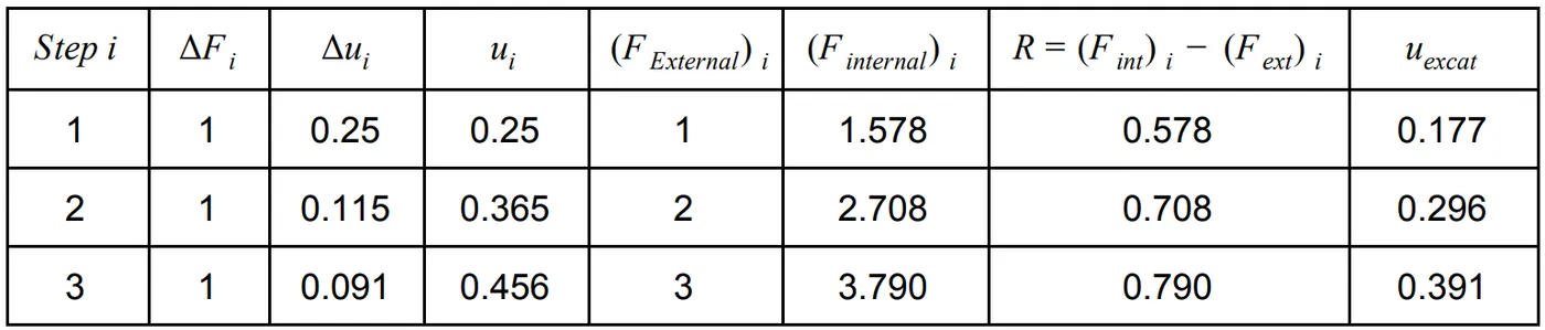
• It is evident from the results that external and internal forces are not in equilibrium because `F_(External)neF_(Internal)`.

Using implicit method:

• An implicit analysis is the same as the explicit analysis, except that at the end of each step Newton-Raphson iterations are used to enforce equilibrium before moving to the next step. Basically, an incremental force is applied to advance the solution forward at the beginning of a step. However, internal forces and external forces will not be in equilibrium unless the stiffness is linear for the given step. Hence, in order to achieve equilibrium, corrections must be made to the displacement. This is accomplished by using Newton-Raphson iterations to minimize the residual, `R(u)=F_(Internal)-F_(External)`. Expanding the residual as a Taylor series about the current displacement `u^j` gives,
• `R^(j+1)=R^j(u^j)+(dR(u^j))/(du)deltau^(j+1)+...=R^j+k(u^j)deltau^(j+1)+...`
• By neglecting higher order terms in the series, setting `R^(j+1)` = 0 and solving for `deltau^(j+1)` the following correction is obtained.
• `deltau^(j+1)=-[k(u^j)]^-1R^j`
• Notice that the iteration variable is `j` and it may take several iterations for the norm of the residual, , to be reduced below the chosen tolerance criteria (for the example below a tolerance of 0.01 is chosen). The implicit analysis proceeds as follows (results are approximate, they are more precise if done in a computer to machine precision):

Step 1:

• At `u_0=0 implies k(u_0)=4` , `DeltaF=1`
• `Deltau_1= (DeltaF)/(k(u_0)`=`1/4=0.25`
• `u_1=u_0+Deltau_1=0.25`
• Checking the residual,
• `F_(External)=DeltaF=1`
• `F_(Internal)=u^3+9u^2+4u=1.578`
• `R^((0))=F_(Internal)-F_(External)=0.578`
• `R^((0))>0.01 implies text(Newton Raphson iterations are necessary)`
• Calculating the correction to `u_1=u_1^((0))`
• `deltau^((1))=-[k(u_1^((0)))]^-1R^((0))=-(8.687)^-1**(0.578)=0.066`
• The updated value of `u_1^((1))=u_1^((0))+deltau^((1))=0.25-0.066=0.184`
• Checking the residual again,
• `F_(External)=DeltaF_=1`
• `F_(Internal)=u^3+9u^2+4u`, Putting (`u=0.184`) gives,
• `F_(Internal)=1.046`
• `R^((1))=F_(Internal)-F_(External)=0.046`
• `R^((1))>0.01 implies text(Newton Raphson iterations are necessary)`
• Calculating the new total correction to `u_1=u_1^((0))`
• `deltau^((2))=deltau^((1))-[k(u_1^((1)))]^-1R^((1))=-0.066-(7.413)^-1**0.046=-0.072`
• The updated value of `u_1^((2))=u_1^((0))+deltau^((2))=0.25-0.072=0.178`
• Checking for the residuals again,
• `F_(External)=DeltaF=1`
• `F_(Internal)=u^3+9u^2+4u` Putting (`u=0.178`) gives,
• `F_(Internal)=1.002`
• `R^((2))=F_(Internal)-F_(External)=0.002`
• `R^(2)<0.01implies text(Newton-Raphson iterations are not necessary)`
• `therefore text(The final value is ) u_1=u_1^((2))=0.178`

Step 2:

• `u_1=0.178impliesk(u_1)=7.299, DeltaF=1`
• `Deltau_2=(DeltaF)/(k(u_1))=1/7.299=0.137`
• `u_2=u_1+Deltau_2=0.178+0.137=0.315`
• Checking the residuals,
• `F_(External)=DeltaF+DeltaF=1+1=2`
• `F_(Internal)=u^3+9u^2+4u=2.184`
• `R^((0))=F_(Internal)-F_(External)=0.184`
• `R^((0))>0.01 implies text(Newton Raphson iterations are necessary)`
• Calculating the corrections to `u_1=u_0^((0))`
• `deltau^((1))=-[k(u_1^((0)))]^-1R^((0))=-(9.967)^-1**0.184=-0.018`
• The updated value of `u_2^((1))=u_1^((0))+deltau^((1))=0.315-0.018=0.297`
• Checking the residuals again,
• `F_(External)=DeltaF+DeltaF=1+1=2`
• `F_(Internal)=u^3+9u^2+4u=2.008`
• `R^((0))=F_(Internal)-F_(External)=0.008`
• `R^(1)<0.01implies text(Newton-Raphson iterations are not necessary)`
• `therefore text(The final value is ) u_2=u_1^((1))=0.297`

Step 3:

• `u_2=0.297impliesk(u_2)=9.6106, DeltaF=1`
• `Deltau_3=(DeltaF)/(k(u_2))=1/9.6106=0.10405`
• `u_3=u_2+Deltau_3=0.297+0.10405=0.40105`
• Checking the residuals,
• `F_(External)=DeltaF+DeltaF+DeltaF=1+1+1=3`
• `F_(Internal)=u^3+9u^2+4u=3.1162`
• `R^((0))=F_(Internal)-F_(External)=0.1162`
• `R^((0))>0.01 implies text(Newton Raphson iterations are necessary)`
• Calculating the corrections to `u_2=u_2^((0))`
• `deltau^((2))=-[k(u_3^((0)))]^-1R^((0))=-(11.701)^-1**0.1162=-0.00993`
• `u_3^((1))=u_3^((0))+deltau^((2))=0.40105-0.00993=0.39112`
• Checking the residuals again,
• `F_(External)=DeltaF+DeltaF+DeltaF=1+1+1=3`
• `F_(Internal)=u^3+9u^2+4u=3.001`
• `R^((0))=F_(Internal)-F_(External)=0.001`
• `R^(1)<0.01implies text(Newton-Raphson iterations are not necessary)`
• `therefore text(The final value is ) u_3=u_3^((2))=0.391`

Table 2: Summary of implicit analysis results

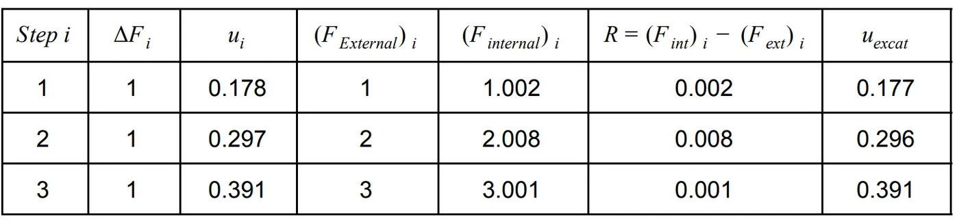
It is evident from the table that the external forces and internal forces are coming into equilibrium.

RESULTS:

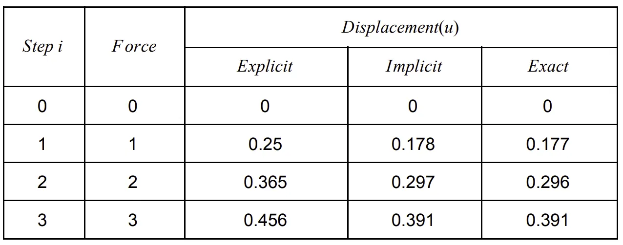
• The given equation have been solved using explicit and implicit methods to find out the variation in displacements and compared with the excat displacement.
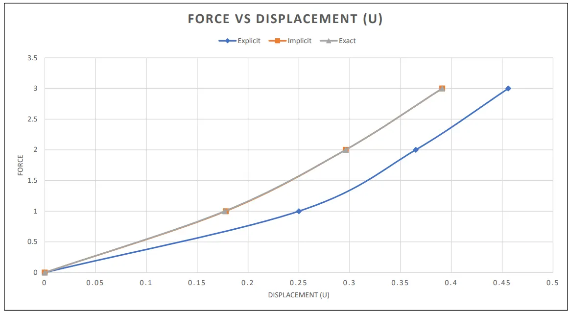
• The values have been tabulated and plotted graph between Force vs Displacement.

Table 3:

Graph:

CONCLUSION:

• It is evident from the plot that the explicit analysis drifts from the exact solution. If 20 increments are used the explicit analysis more closely follows the exact solution. However, even with more increments the explicit analysis still drifts from the exact solution. The drift from the exact solution illustrates the lack of equilibrium between the internal and external forces. To correct for this problem an implicit analysis is required. The Newton-Raphson iterations correct the incremental steps so that they land on the exact solution according to the specified tolerance also an excellent agreement is achieved with just 3 increments. From the graph we can see that the implicit and excat results lie very close to each other.
• Here the problem is considered only for the load control scheme. For other schemes such as displacement control, arc length control etc can also be carried out with this method.