Week - 9 Material Modeling from Raw Data

Objective

To model a material using the given true stress-strain curve of graphite iron casting and validate the data by creating either a MAT_024 or MAT_018 material to the dogbone specimen following other objectives as well which are shown below.

• Extraction of data from the diagram.
• Clean the data and match it with the original data.
• Use the given unit system (kg-mm-ms).
• Process the data and create the material as demonstrated
• Use the material model with a dogbone specimen and validate the same.

Introduction

• To model a linear behavior of material only three independent parameters are required to calculate stress and strains. These three parameters are young modulus, poisons ratio, and density. The linear relation is as per the straight line is described only by the slope ie youngs modulus. It is when the material enters the non-linear zone after the yield strength limit, the curve needs to be described using different non-linear functions according to the way the material behaves under different types of loading.

Elasto-plastic Materials

• Stress-strain for structural steel will consist of the elastic and perfectly plastic region. . We call this kind of material elastoplastic material.
• Bilinear stress-strain diagram having different slopes is sometimes used to approximate the general nonlinear diagrams. This will include strain hardening.

*MAT_018 (*MAT_POWER_LAW_PLASTICITY)

• This is Material Type 18. This is an isotropic plasticity model with rate effects that uses a power-law hardening rule.
• `sigma_(y)= kepsilon^n`
• `sigma_y`: Yield stress
  `epsilon`: Total strain
  k Strength coefficient.
  n Hardening exponent

*MAT_024 (*MAT_PIECEWISE_LINEAR_PLASTICITY)

• This is Material Type 24, which is an elastoplastic material with arbitrary stress versus strain curve and arbitrary strain rate dependency can be defined.
• Here failure based on a plastic strain or a minimum time step size can be defined.
• The stress-strain behavior may be treated by a bilinear stress-strain curve by defining the tangent modulus, ETAN. Alternately, a curve of effective stress vs effective plastic strain may be defined by a curve ID (LCSS). With this LCSS, a continuous smooth stress-strain curve with small linear steps can be achieved.
• So here we have the experimental data for the stress-strain curve, so using this card will be better to model.

Procedure

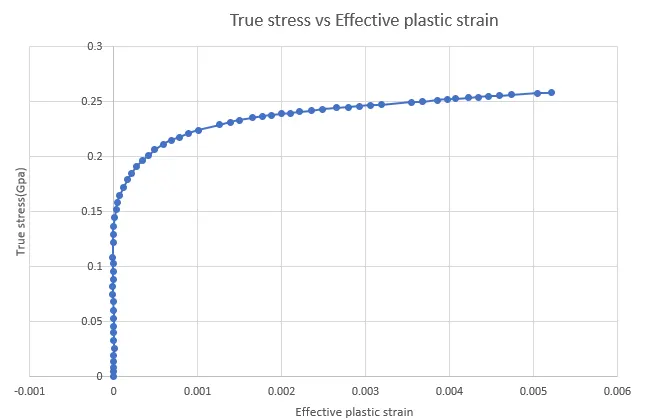
• From the given graph the second curve was selected and extracted the data points using a data digitizer. These values were then copied to an excel sheet.

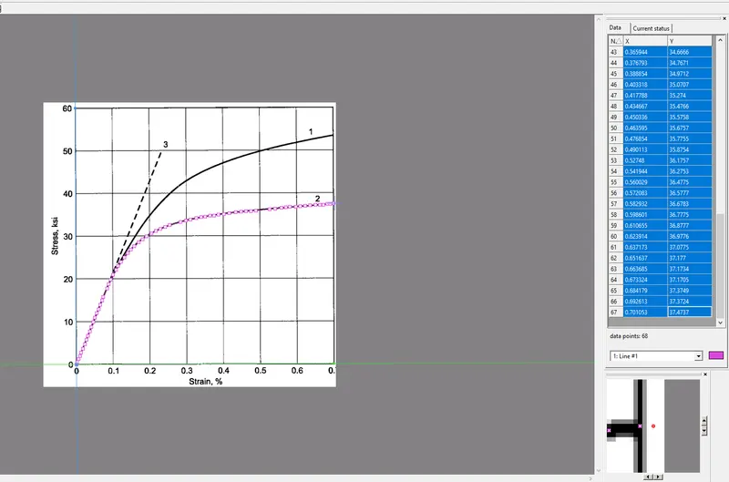
• After extracting the data, the values for effective plastic strain and true stress were found out.
• The given stress value was in ksi and its been converted Gpa by multiplying it with 0.00689476.
• Effective plastic strain =True strain-(True stress/E).
• A graph has been plotted between true stress and true strain.

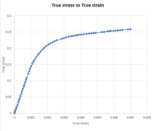
• By observing the graph it's seen that the curve is smooth and further curve fitting is not needed. Here we have taken lots of points while extracting the curve data from the digitizer. If only a few points were been taken into consideration there might be a need for curve fitting.

• Now the .k file of the given model was opened in Ls-Prepost.

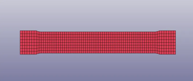
Defining material and section to the part

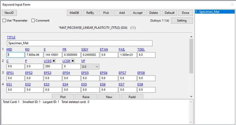
• *MAT_PIECEWISE_LINEAR_PLASTICITY card from keyword manager was used to specify the material to the given dogbone specimen by assigning the values as given below.
• The value for elastic modulus was given as 20.9E+06 psi and it been converted to GPa.
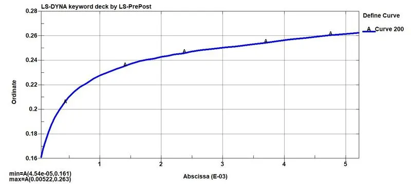
• Before assigning the values in this material card, We need to find out the yield stress from the graph stress-strain graph using the method given below. Also, a curve has to be defined for LCSS taking all the points after the yield point.
• If the load curve is defined using LCSS, then there is no need to assign ETAN (Tangent modulus).

Finding out the yield point

• The value of effective plastic strain is the integral of stepwise increments of plastic deformation for a period of time t. Effective plastic strain is always used as an erosion criterion to remove damaged elements in a numerical simulation.
• True stress vs effective plastic strain plot was plotted to find the yield point and it was seen that the material behavior elastically up to yield point and then its undergo plastic deformation. Therefore the point where the non-linearity begins was chosen as the yield point for this case and the yield stress was found to be 0.1522260 GPa.

• A curve was also defined by using yield point and the points after that in order to define load curve(LCSS) can be assigned. This can be easily done using Notepad++.

• A shell section card with a thickness of 1.5mm was also created and these cards along with the material card were assigned to the part id.

Boundary conditions

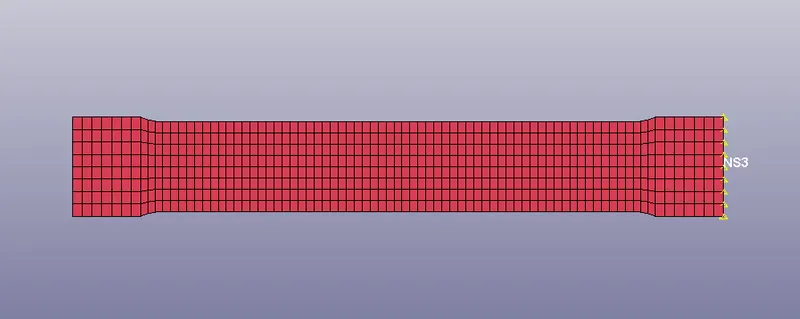
• The displacement was given to the end nodes using *BOUNDARY_PRISCRIBED_MOTION_SET. The value for the displacement was calculated as follows.

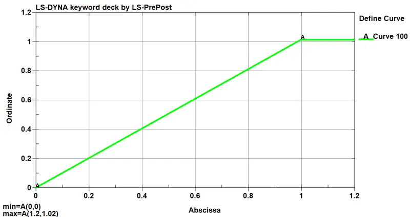
• True strain from the given data was found to be 0.00701053.
• Displacement=True strain * Initial dimension(145mm)=1.01652mm.
• This value has been assigned to the load curve scale factor also a load curve has been created to define the displacement.

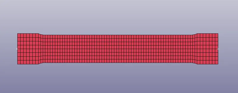
• The nodes at the other end of the model are fixed in all DOF except at translation along the y-axis using single point constraint(SPC).

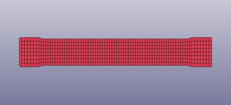
• Also, two more nodes are constrained only in the y-direction as shown in the figure below to describe the actual behavior of the model.

Control cards for implicit analysis.

• *CONTROL_IMPLICIT_GENERAL: The keyword makes sure that the analysis will start in an implicit manner since the default analysis mode for ls dyna is explicit. Here the IMFLAG is set to 1 to activate the implicit analysis.
• *CONTROL_IMPLICIT_AUTO: Used to change the time step for the given problem. In implicit the time step can be changed since its unconditionally stable but in explicit analysis the time step is the condition beyond a certain value. Here IAUTO value was kept as one.

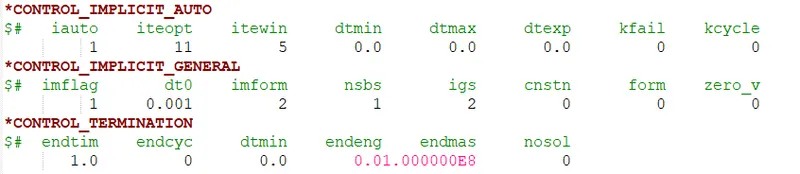
• Apart from this other cards such as *DATA_BASE_EXTENT_BINARY, *DATABASE_ASCII, and BINARY_D3PLOT were created to get the required outputs.
• The end time was defined as one using the *CONTROL_TERMINATION card.

Model check-up and running the simulation.

• The model is checked for any errors and if any error occurs it should be corrected further.
• The .k file is been saved and ran using LS-DYNA manager.
• If Normal termination is showed after running the file, it's then ready to do the post-processing.

Results

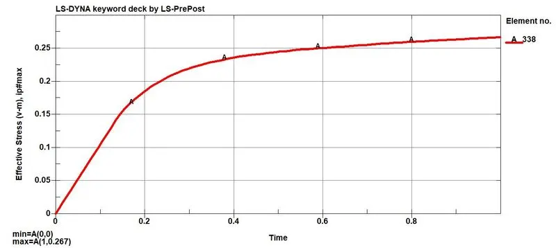
Effective stress

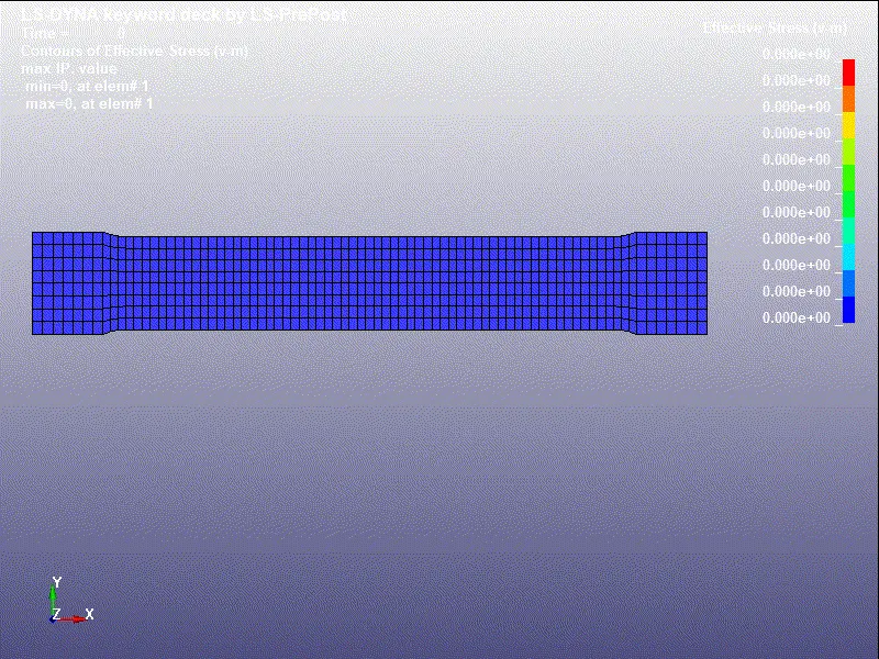
• The above plot shows the effective stress (Von-Mises stress) when the specimen was subjected to a tensile test. The maximum stress value was shown as 0.2726 GPa which lies in the middle region of the specimen. Hence the maximum stress observed from this test was more than the yield stress defined, the undergo yielding and a plastic deformation was observed.

Effective plastic strain

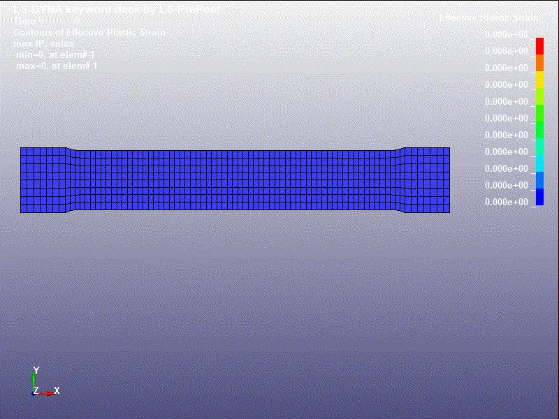
• This shows the effective plastic strain behavior of the material when subjected to a tensile load. The maximum stain was seen at the middle portion of the specimen and it was found to be 7.250e-3.
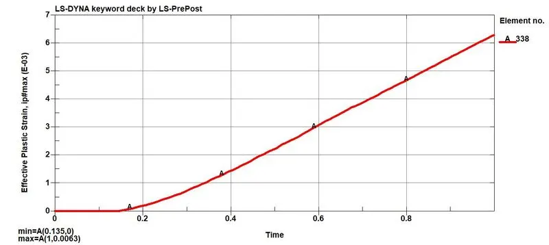
• The plot below shows the variation of the effective stress with respect to time.

Validation of stress-strain curve

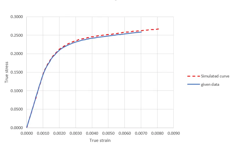
• From the post-processing data, we get a curve between effective plastic stress and lower lpt x-strain which is shown below.

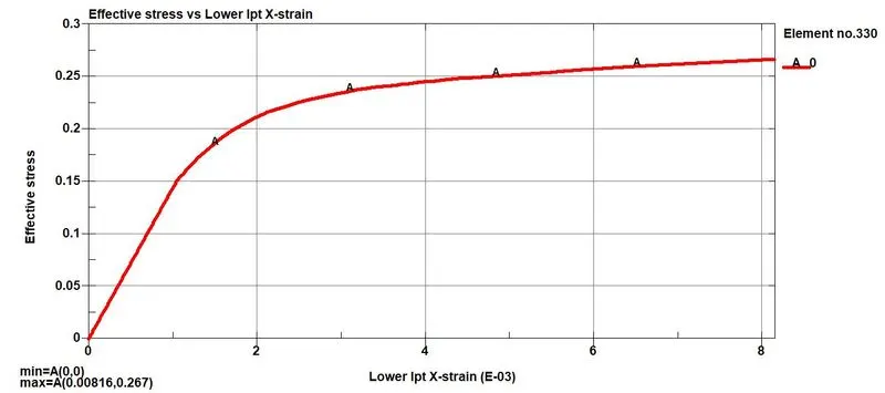
• All the values for the effective stress and the lower lpt x-strain can be extracted after plotting by saving the graph as .csv file.
• The simulated curve was then compared with the experimental data to validate it using the MAT_24 material card. It can be observed that the simulated curve almost fits with the experimental data. But the result that got from the simulated data was a little bit more than that of experimental data.

Conclusion

• Material modeling for the given specimen has been done with reference to the experimental data and validated with the MAT_24 material card.

process and failures

• For a ductile material, the change from elastic region to plastic region occurs gradually. So it's difficult to find out the yield point exactly. Its been calculated by the 0.2% offset method for the given material. This can be done by constructing a parallel line from the linear stress-strain curve. The intersection point of the newly constructed line to the stress-strain curve gives the yield point and this value can be taken while assigning the material card for this model.

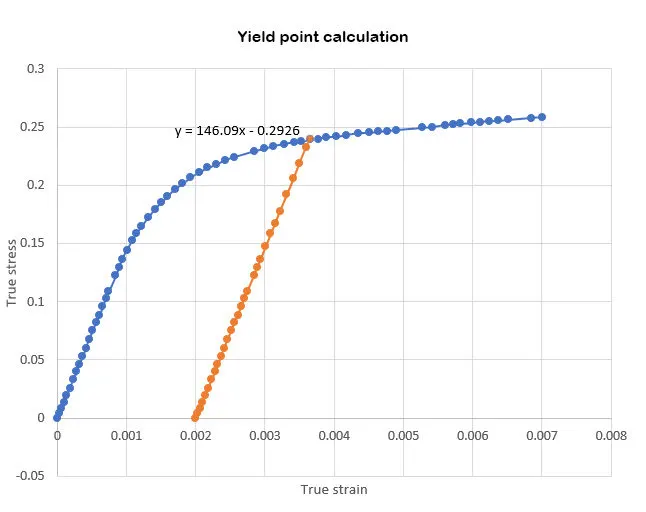
• The value got for yield stress from the graph using this method was found to be 0.240585221GPa.
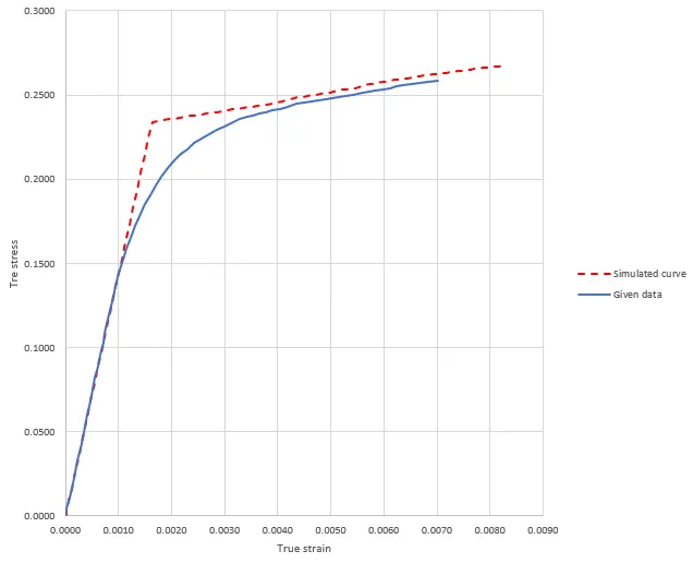
• But while using this method the simulated curve deviates much from the given experimental data. Therefore other method was followed as discussed above which gives a fit to the given experimental data curve.

• When copying the data from excel sheet to Notepad++ there were problems with the alignment which results in the plotting of an improper curve by the software.
• The stress-strain data got after the simulation was again converted to true stress-strain data which is not necessary since ls-dyna given the output in the form of true stress and strain only.

.............................................................................................................................................................................................................

File: https://drive.google.com/drive/folders/1gNA2l3zzLPpNbZRo6uKla1RzNweENK29?usp=sharing