Week 2 Air standard Cycle

Aim:

To create a PV diagram for the otto cycle, with plots and air standard effeciency of the engine.

Otto cycle:

The Otto cycle is often plotted on a pressure-volume diagram (pV diagram) and a temperature-entropy diagram (Ts diagram). When plotted on a pressure-volume diagram, the isochoric processes follow the isochoric lines for the gas (the vertical lines), adiabatic processes move between these vertical lines, and the area bounded by the complete cycle path represents the total work that can be done during one cycle.

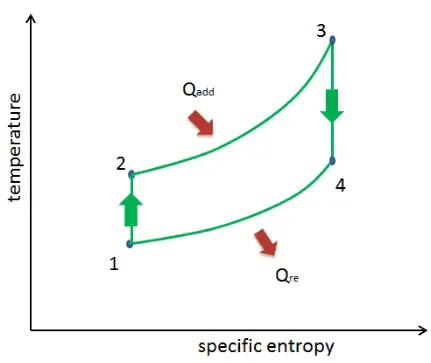
The temperature-entropy diagram (Ts diagram) in which the thermodynamic state is specified by a point on a graph with specific entropy (s) as the horizontal axis and absolute temperature (T) as the vertical axis. Ts diagrams are a useful and common tool, particularly because it helps to visualize the heat transfer during a process. For reversible (ideal) processes, the area under the T-s curve of a process is the heat transferred to the system during that process

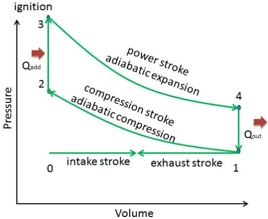
pV diagram of Otto Cycle.
The area bounded by the complete cycle path represents the total work that can be done during one cycle.

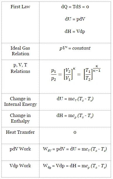
Isentropic Process
An isentropic process is a thermodynamic process in which the entropy of the fluid or gas remains constant. It means the isentropic process is a special case of an adiabatic process in which there is no transfer of heat or matter. It is a reversible adiabatic process. The assumption of no heat transfer is very important since we can use the adiabatic approximation only in very rapid processes.

Isentropic Process and the First Law
For a closed system, we can write the first law of thermodynamics in terms of enthalpy:

dH = dQ + Vdp

or

dH = TdS + Vdp

Isentropic process (dQ = 0):

dH = Vdp → W = H₂ – H₁ → H₂ – H₁ = C_p (T₂ – T₁) (for ideal gas)

Isentropic Process of the Ideal Gas

The isentropic process (a special case of the adiabatic process) can be expressed with the ideal gas law as:

pV^κ = constant

or

p₁V₁^κ = p₂V₂^κ

in which κ = c_p/c_v is the ratio of the specific heats (or heat capacities) for the gas. One for constant pressure (c_p) and one for constant volume (c_v). Note that, this ratio κ = c_p/c_v is a factor in determining the speed of sound in a gas and other adiabatic processes.

Isothermal Process
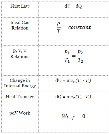
An isochoric process is a thermodynamic process in which the volume of the closed system remains constant (V = const). It describes the behavior of gas inside the container that cannot be deformed. Since the volume remains constant, the heat transfer into or out of the system does not the p∆V work but only changes the system’s internal energy (the temperature).

Isochoric Process and the First Law

The classical form of the first law of thermodynamics is the following equation:

dU = dQ – dW

In this equation, dW is equal to dW = pdV and is known as the boundary work. Then:

dU = dQ – pdV

An isochoric process and the ideal gas, all of the heat added to the system, will increase the internal energy.

Isochoric process (pdV = 0):

dU = dQ (for ideal gas)

dU = 0 = Q – W → W = Q (for ideal gas)

Isochoric Process of the Ideal Gas

The isochoric process can be expressed with the ideal gas law as:

or

On a p-V diagram, the process occurs along a horizontal line with the equation V = constant.

Derivation for air standard effeciency of otto-cycle:

https://old.amu.ac.in/emp/studym/7331.pdf

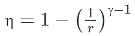
R = compression ratio
Gamma = Ratio of specific heat

Code:

• Coding has been done in Sublime text editor 3 using python as the scripting language.
• The code is split into 2 parts where the first part contains a function to calculate the Volume of the engine cylinder. The second part deals wirth the value initialisation and function call and ends with plotting the values using the matplotlib.pyplot library.
• The function starts with passing most relevant data that is important for calculation within the function. Crank radius, Clearemce volume, swept volume, scrank start angle and crank end angle in radians, number of data points, change in crank angle etc are provided within the function which has been named 'engine_kinematics'.
• An empty array for storing volume has been initialised before the for loop, the for loop calculates the theta values or the change in theta for each interation, then the for loop proceeds to calculate the value for swept volume using an emperical relation and the append command enters these values into the swept volume empty array.
• The second part deals with the function call, calculation, initialisation of useful variables and plotting of values.
• Thermodynamic properties such as pressure, temperature, volume are calcuated for each stroke of the engine. Isentropic relations have beenused to produce a curve plot rather than a straight line.
• At the adiabatic compression and expansion volume and pressure values have been calculated and stored in an array for lotting later.
• The air standard effeciency of the otto cycle has been calcuated using the formula and the plots are plotted using the matplotlib library.

"""otto cycle simulator"""

import math
import matplotlib.pyplot as plt


def engine_kinematics(bore, stroke, con_rod, cr, start_crank, end_crank):


    a = stroke/2 
    R = con_rod/a
    V_s = math.pi*(1/4)*pow(bore, 2)*stroke
    V_c = V_s/(cr - 1)

    # angle  
    sc = math.radians(start_crank)  # sc = start crank: crank angle 0 and piston at top dead center: converting the degrees into radians
    ec = math.radians(end_crank)  # crank angle 0 and piston at bottom dead center: converting the degrees into radians

    num_values=50
    dtheta = (ec - sc)/(num_values-1)

    # to store volume array
    V=[]

    #to start crank angle array
    for i in range(0, num_values):
        theta = sc + i*dtheta    

        term1 = 0.5*(cr-1)
        term2 = R + 1 - math.cos(theta)
        term3 = pow(R, 2) - pow(math.sin(theta), 2)
        term3 = pow(term3, 0.5)

        V.append((1 + term1 * (term2-term3))*V_c)
    return V 


# inputs
p1 = 101325
t1 = 500
t3 = 2300
gamma = 1.4

# geometric parameters
bore = 0.1
stroke = 0.1
con_rod = 0.15 # connecting rod
cr = 12 # compression ratio

# volume computation
v_s = (math.pi/4)*pow(bore, 2)*stroke # stroke volume
v_c = v_s/(cr-1)                      # clearence volume

# volume at state 1
v1 = v_c + v_s                        


# state point 2 - compression cycle
v2 = v_c 
p2 = p1*pow(v1, gamma)/pow(v2, gamma)

# temperature at state point 2 
rhs_two = p1*v1/t1
t2 = p2*v2/rhs_two

# for compression: engine_kinematics(bore, stroke, con_rod, cr, 0, 180) # for expansion stroke the crank angle goes from 0 to 180
V_compression = engine_kinematics(bore, stroke, con_rod, cr, 180, 0)
constant = p1*pow(v1, gamma)
P_compression = []

for v in V_compression:
    P_compression.append(constant/pow(v, gamma))
print(P_compression)


# volume of state 3
v3 = v2
rhs_three = p2*v2/t2
p3 = rhs_three*t3/v3
# print(p3 > p2)

# for compression: engine_kinematics(bore, stroke, con_rod, cr, 0, 180)
V_expansion = engine_kinematics(bore, stroke, con_rod, cr, 0, 180)
constant = p3*pow(v3, gamma)
P_expansion = []

for v in V_expansion:
    P_expansion.append(constant/pow(v, gamma))
print(P_expansion)

# state point 4
v4 = v1
p4 = p3*pow(v3, gamma)/pow(v4, gamma)
t4 = p4*v4/rhs_two

# Air standard effeciency:
eta = (1-pow((1/cr), (gamma -1)))*100 
print('Air standard effeciency of otto cycle = ', eta)


plt.plot([v2, v3],[p2, p3], label = 'Igition')
plt.plot(V_compression, P_compression, label = 'Power stroke: Adiabatic expansion')
plt.plot(V_expansion, P_expansion, label = 'Compression stroke: Adiabatic expansion')
plt.plot([v4, v1],[p4, p1], label = 'Exhaust')
plt.legend()
plt.xlabel('Volume [m^3]')
plt.ylabel('Pressure [Pa]')
plt.show()

Result and plot:

Air standard effeciency of otto cycle = 62.98928275128466%

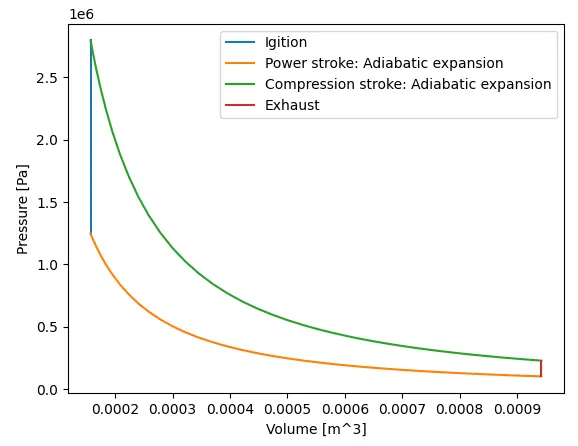
It can be clearly seen that the Constant volume plot has been obtained distinctly, and each stroke has been colored in a unique fashion to visualise data better.
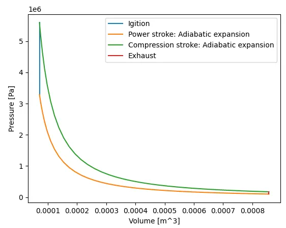
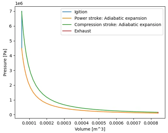
Below are the change in plot shape that happens when we change the compression ratios of the otto cycle.
The otto cycle's exhaust stroke is sensitive to the change in the value of clearence volume.

PV diagram for compression ratio: 6

PV diagram for compression ratio: 12

PV diagram for compression ratio: 15

Project link:

https://skill-lync.com/student-projects/week-2-air-standard-cycle-335

Reference:

https://www.nuclear-power.com/nuclear-engineering/thermodynamics/thermodynamic-cycles/otto-cycle-otto-engine/otto-cycle-pv-ts-diagram/

https://www.aboutmech.com/2016/01/efficiency-of-ic-engine.html