Week 5.1 - Mid term project - Solving the steady and unsteady 2D heat conduction problem

Thermal/Heat Conduction :

Heat conduction was defined as the transfer of thermal energy from the more energetic particles of a medium to the adjacent less energetic ones. It was stated that conduction can take place in liquids and gases as well as solids provided that there is no bulk motion involved.
Although heat transfer and temperature are closely related, they are of a different nature. Unlike temperature, heat transfer has direction as well as magnitude, and thus it is a vector quantity.

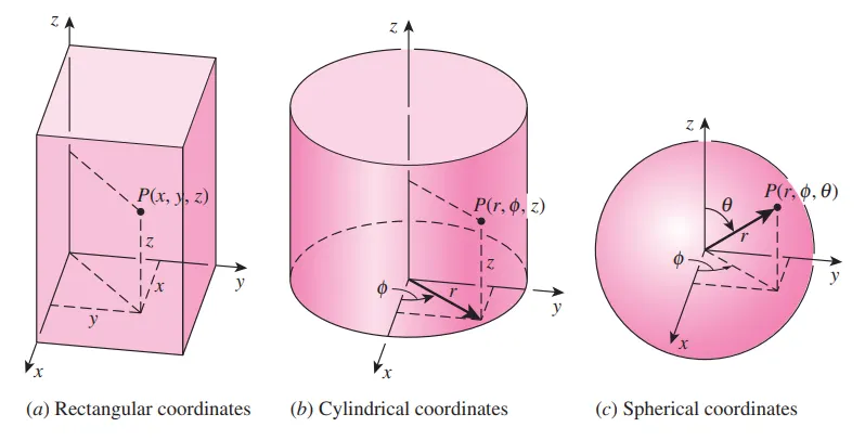
The location of a point is specified as (x, y, z) in rectangular coordinates, as (r, `phi`, z) in cylindrical coordinates, and as (r, `phi`, `theta`) in spherical coordinates,
where the distances are in x, y, z
r is the radius
and angles `phi` and `theta`.

Then the temperature at a point (x, y, z) at time t in rectangular coordinates is expressed as T(x, y, z, t).
The notation just described is also used to identify the variables involved in a heat transfer problem. For example, the notation T(x, y, z, t) implies that the temperature varies with the space variables x, y, and z as well as time.

Heat transfer problems are often classified as being steady (also called steadystate) or transient (also called unsteady).
The term steady implies no change with time at any point within the medium, while transient implies variation with time or time dependence.
With respect to mass balance, steady state occurs whenever the mass flow into a system is equal to the mass flow out of the system, where accumulation and net generation in the system is zero.
Therefore, the temperature or heat flux remains unchanged with time during steady heat transfer through a medium at any location, although both quantities may vary from one location to another.

We have considered a 1m x 1m square slab for simulating the heat flow with boundary conditions as stated below :

Top Boundary = 600 K
Bottom Boundary = 900 K
Left Boundary = 400 K
Right Boundary = 800 K

The initial temprature to all the nodes apart from the boundary values is 300K.

The corner nodes of the matrix is an average of the value of the 2 adjacent elements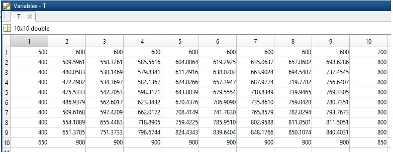

For example : The matrix element 1x1 is 500 ,

which is the average of the 2 adjacent elements of corner element 500
ie.,`(400+600)/2=500`

This applies to all the corner elements of the matrix and is done to get finer values over the graph.

Multidimensional Heat Transfer :

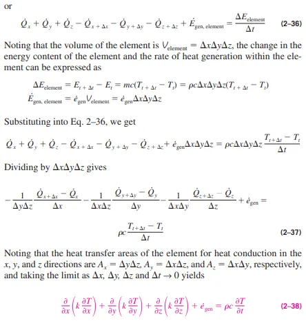
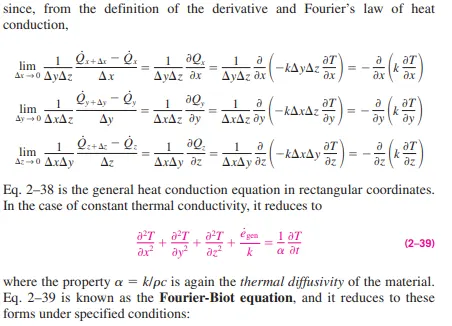
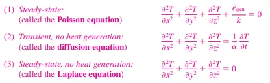
Heat transfer problems are also classified as being one-dimensional, twodimensional, or three-dimensional, depending on the relative magnitudes of heat transfer rates in different directions and the level of accuracy desired. In the most general case, heat transfer through a medium is three-dimensional. That is, the temperature varies along all three primary directions within the medium during the heat transfer process. The temperature distribution throughout the medium at a specified time as well as the heat transfer rate at any location in this general case can be described by a set of three coordinates such as the x, y, and z in the rectangular (or Cartesian) coordinate system.

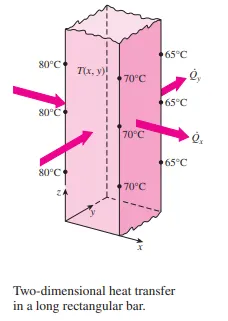
Rectangular coordinates :

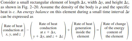
Steady state 2d conduction :

Discretization:

`alpha*[(del^2T)/(delx^2)+(del^2T)/(dely^2)]=0`
`(del^(2)T)/(delx^2)=[T_(i-1,j)-2*T_(i,j)+T_(i+1,j)]/(Deltax^2)`

`(del^(2)T)/(dely^2)=[T_(i,j-1)-2*T_(i,j)+T_(i,j+1)]/(Deltay^2)`

Here, i & j are spatial coordinates in the matrix

`[T_(i-1,j)-2T_(i,j)+T_(i+1,j)]/(Deltax^2)+[T_(i,j-1)-2*T_(i,j)+T_(i,j+1)]/(Deltay^2)=0`

`2*T_(i,j)/[Deltax^2]+2*T_(i,j)/[Deltay^2]=[T_(i-1,j)+T_(i+1,j)]/(Deltax^2)+[T_(i,j-1)+T_(i,j+1)]/(Deltay^2)`

`T_(i,j)*(2/(Deltax^2)+2/(Deltay^2))=[T_(i-1,j)+T_(i+1,j)]/(Deltax^2)+[T_(i,j-1)+T_(i,j+1)]/(Deltay^2)`

From here we can calculate 'K'
`K=2*((Deltax)^2+(Deltay)^2)/((Deltax)^2*(Deltay)^2)`

so,

`T_(i,j)*K=[T_(i-1,j)+T_(i+1,j)]/(Deltax^2)+[T_(i,j-1)+T_(i,j+1)]/(Deltay^2)`

CODE :

clear all
close all
clc

nx=10;
ny=nx;

L=1;

T=300*ones(nx,ny)

T_left=400;
T_top=600;
T_right=800;
T_bottom=900;

% boundary conditions
% u(:,1)means that the elements of first column is of 400
T(:,1)=T_left;
% (1,:)means that the row elements of all columns in the first row is 600
T(1,:)=T_top;
T(:,end)=T_right;
T(end,:)=T_bottom;

% for better corner values we take the average of the 2 adjacent values to
% the corner value
T(1,1)=(T(1,2)+T(2,1))/2;
T(1,end)=(T(1,ny-1)+T(2,ny))/2;
T(end,1)=(T(nx-1,1)+T(nx,2))/2;
T(end,end)=(T(nx,ny-1)+T(nx-1,ny))/2;

Told=T;

x=linspace(0,L,nx);
y=linspace(0,L,ny);

dx=x(2)-x(1);
dy=y(2)-y(1);
K=2*((dx)^2+(dy)^2)/((dx)^2*(dy)^2);

iterative_solver=1

error=9e9;
tol=1e-4;

omega=1.1;

if iterative_solver==1
jacobi_iter=1;
tic
while(error>tol)

for i=2:nx-1
for j=2:ny-1

T(i,j)=(1/K)*((Told(i-1,j)+Told(i+1,j))/(dx^2)+(Told(i,j-1)+Told(i,j+1))/(dy^2));

end
end
% had to use (max(max(abs(Told-T)))
error=(max(max(abs(Told-T))));
jacobi_iter=jacobi_iter+1
Told=T;

figure(1)
[A,B]=contourf(x,y,T);
set(gca,'ydir','reverse')
colorbar
colormap(jet)
clabel(A,B)
title_text=sprintf('Jacobi Iteration number=%d',jacobi_iter);
xlabel('X - 1 meter')
ylabel('Y - 1 meter')
title(title_text)
pause(0.0001)

end
toc
end

% % % % % % % % % % % % % % % % % %
if iterative_solver==2

gs_iter=1;
tic
while(error>tol)

for i=2:nx-1
for j=2:ny-1

T(i,j)=(1/K)*((T(i-1,j)+Told(i+1,j))/(dx^2)+(T(i,j-1)+Told(i,j+1))/(dy^2));

end
end
% had to use (max(max(abs(Told-T)))
error=(max(max(abs(Told-T))));
gs_iter=gs_iter+1
Told=T;

figure(2)
[C,D]=contourf(x,y,T);
set(gca,'ydir','reverse')
colorbar
clabel(C,D)
colormap(jet)
title_text=sprintf('GS Iteration number=%d',gs_iter);
xlabel('X - 1 meter')
ylabel('Y - 1 meter')
title(title_text)
pause(0.03)
end
toc
end

% % % % % % % % % % % % % % % % % % % % % % % % %
if iterative_solver==3

sor_iter=1;
tic
while(error>tol)

for i=2:nx-1
for j=2:ny-1

T(i,j)=(1-omega)*(Told(i,j))+(omega)*((1/K)*((T(i-1,j)+Told(i+1,j))/(dx^2)+(T(i,j-1)+Told(i,j+1))/(dy^2)));

end
end
% had to use (max(max(abs(Told-T)))
error=(max(max(abs(Told-T))));
sor_iter=sor_iter+1
Told=T;

figure(3)
[E,F]=contourf(x,y,T);
set(gca,'ydir','reverse')
colorbar
clabel(E,F)
colormap(jet)
title_text=sprintf('SOR Iteration number=%d',sor_iter);
xlabel('X - 1 meter')
ylabel('Y - 1 meter')
title(title_text)
pause(0.03)
end
toc
end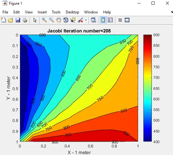

Discussion :

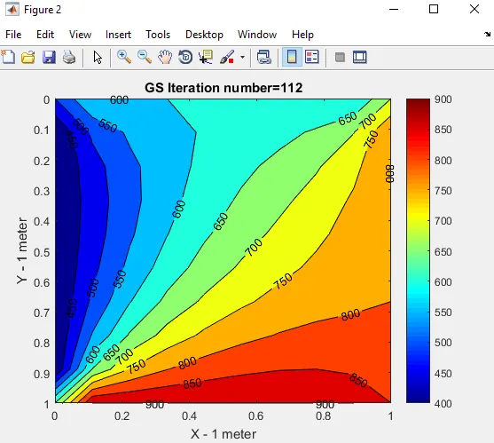
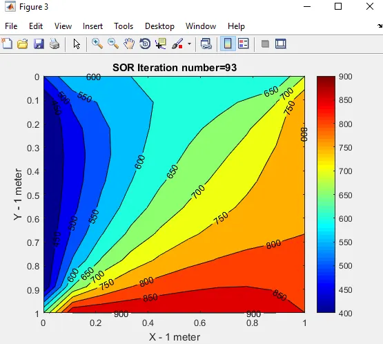
1.The code is structured in such a way that all the 3 iterative solvers can be run from the same code by changing the iteration number .
Type 1 as the iteration number for the plot of Jacobi .
Type 2 as the iteration number for the plot of Gauss Siedel.
Type 3 as the iteration number for the plot of Successive Over Relaxation .

2.A square domain is chosen of dimension 1m .The domain is further discretised into a number of divisions along x & y axis and hence nx=ny=10
3.The tempratures on the walls of the domain is specified as boundary conditions ,the initial temprature to all the nodes apart from the boundary values is 300K.
Top Boundary = 600 K
Bottom Boundary = 900 K
Left Boundary = 400 K
Right Boundary = 800 K
4.Further the matrix's corner elements are average values of the adjacent elements and this is done to get better corner values while plotting the Temprature values .
5.A matrix copy for T is generated by equating T to Told which we will be using in the code for value updation.
6.'dx' & 'dy' are found out from the difference of the indeces of 'x' & 'y' respectively .
7.'K' a constant is computed initially for further calculations by the program .
8.omega for SOR is declared,error & tolerance values are stated for the code to enter the while loop further in the code .
9.Iterative_solver= '?' gives the condition for matlab to choose any one among the three iterative solvers .
10. The 'if' statement verifies the value at iterative_solver to either ignore or run a set of code below the if command , if the number on the RHS of the iterative_solver matches with the 'if' command then the code runs to produce an output .
11. The while loop allows the code to run until the criteria error>tol.
12.The 2 'for loops' are for the code to calculate i & j positionn values in the matrix.
13.Jacobi , Gauss siedel or SOR gets executed for a given number iterations till the solution converges .
14.error is caluclated for the code to again enter the while loop until solution converges.
15.T values are updated into the Told matrix for use later in the for loop .
16.The code uses contourf command to get a fully filled contour of the Temprature values in the graph .
17.''set(gca,'ydir','reverse')'' reverses the y axis for accurate output because Tbottom is 900K
18.colorbar gives the small vertical bar like scale for Temprature ranges generated in the code .
19.colormap(jet) is used to get distinct rgb colors in the graph .
20.clabel is used to label the temprature values on the graph in real time for every iteration .
21.title_text is used to display iteration values on the graph & also doubles as the code line uswed to write title of the graph .

Transient state : Explicit

`(delT)/(delt)=alpha*[(del^2T)/(delx^2)+(del^2T)/(dely^2)]`

Discretization:
`(del^(2)T)/(delx^2)=[T_(i-1,j)-2**T_(i,j)+T_(i+1,j)]/(Deltax^2)`

`(del^(2)T)/(dely^2)=[T_(i,j-1)-2*T_(i,j)+T_(i,j+1)]/(Deltay^2)`

`(delT)/(delt)=[T_(i,j)^(n+1)-T_(i,j)^(n)]/(Deltat)`

Here, i & j are spatial coordinates in the matrix

here ,
`K1=alpha*(Deltat)/(Deltax^2)`

`K2=alpha*(Deltat)/(Deltay^2)`

`[T_(i,j)^(n+1)-T_(i,j)^(n)]/(Deltat)=alpha *[[T_(i-1,j)-2*T_(i,j)+T_(i+1,j)]/(Deltax^2)+[T_(i,j-1)-2*T_(i,j)+T_(i,j+1)]/(Deltay^2)]^n`

`[T_(i,j)^(n+1)-T_(i,j)^(n)]=Deltat*alpha *[[T_(i-1,j)-2*T_(i,j)+T_(i+1,j)]/(Deltax^2)+[T_(i,j-1)-2*T_(i,j)+T_(i,j+1)]/(Deltay^2)]^n`

`T_(i,j)^(n+1)=T_(i,j)^(n)+Deltat*alpha *[[T_(i-1,j)-2*T_(i,j)+T_(i+1,j)]/(Deltax^2)+[T_(i,j-1)-2*T_(i,j)+T_(i,j+1)]/(Deltay^2)]^n`

`T_(i,j)^(n+1)=T_(i,j)^n+(Deltat*alpha)/(Deltax^2)*(T_(i-1,j)+T_(i+1,j))^n+(Deltat*alpha)/(Deltay^2)*(T_(i,j-1)+T_(i,j+1))^n`

`T_(i,j)^(n+1)=T_(i,j)^n+K1*[T_(i-1,j)-2*T_(i,j)+T_(i+1,j)]^n+K2*[T_(i,j-1)-2*T_(i,j)+T_(i,j+1)]^n`

CODE :

% transient explicit 

clear all
close all
clc

nx=10;
ny=nx;

L=1;

T=300*ones(nx,ny)

T_left=400;
T_top=600;
T_right=800;
T_bottom=900;

% boundary conditions
% u(:,1)means that the elements of first column is of 400
T(:,1)=T_left;
% (1,:)means that the row elements of all columns in the first row is 600
T(1,:)=T_top;
T(:,end)=T_right;
T(end,:)=T_bottom;

% for better corner values we take the average of the 2 adjacent values to
% the corner value
T(1,1)=(T(1,2)+T(2,1))/2;
T(1,end)=(T(1,ny-1)+T(2,ny))/2;
T(end,1)=(T(nx-1,1)+T(nx,2))/2;
T(end,end)=(T(nx,ny-1)+T(nx-1,ny))/2;

Told=T;
T_previous=T;

x=linspace(0,L,nx);
y=linspace(0,L,ny);

alfa=1.4;

dx=x(2)-x(1);
dy=y(2)-y(1);
dt=0.001;

K1=alfa*dt/(dx)^2;
K2=alfa*dt/(dy)^2;
CFL=K1+K2
% K=2*((dx)^2+(dy)^2)/((dx)^2*(dy)^2);


error=9e9;
tol=1e-4;

omega=1.1;


iter=1;

% here time loop isnt required because its converging before the time
% loop??not sure 
tic
  for nt=1:1400  
while(error>tol)
    
    for i=2:nx-1
        for j=2:ny-1
            
            T(i,j)=T_previous(i,j)+K1*(T_previous(i-1,j)-2*T_previous(i,j)+T_previous(i+1,j))+K2*(T_previous(i,j+1)-2*T_previous(i,j)+T_previous(i,j-1));

        end
    end
    
%    had to use (max(max(abs(Told-T))) 
     error=(max(max(abs(T_previous-T))));
    iter=iter+1
    
    T_previous=T;
      figure(1)        
[q,w]=contourf(x,y,T)
colorbar
clabel(q,w)
colormap(jet)
set(gca,'ydir','reverse')
xlabel('X - 1 meter')
ylabel('Y - 1 meter')
title_text=sprintf('TRANSIENT EXPLICIT : Iteration number=%d',iter);
title(title_text)
pause(0.0000003)
end

end  
toc

Discussion :

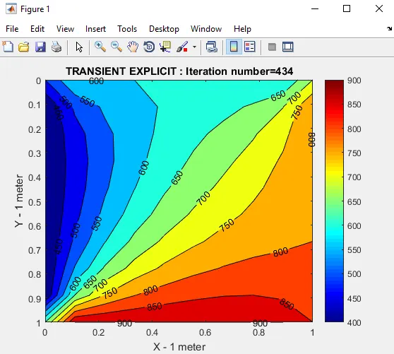
1.The code is structured in such a way that all the iterative solver can run by updation of values from the previous iteration ie.,(n) to find out values at the next time step ie., (n+1).
2.A square domain is chosen of dimension 1m .The domain is further discretised into a number of divisions along x & y axis and hence nx=ny=10
3.The tempratures on the walls of the domain is specified as boundary conditions ,the initial temprature to all the nodes apart from the boundary values is 300K.
Top Boundary = 600 K
Bottom Boundary = 900 K
Left Boundary = 400 K
Right Boundary = 800 K
4.Further the matrix's corner elements are average values of the adjacent elements and this is done to get better corner values while plotting the Temprature values .
5.A matrix copy for T is generated by equating T to Told which we will be using in the code for value updation.
6.'dx' & 'dy' are found out from the difference of the indeces of 'x' & 'y' respectively .
7.'K1 ,K2 & CFL' which are constants are computed initially for further calculations by the program ,here CFL is a key factor in maintaining the stability of the code .
8.alpha values are specified keeping in mind the CFL value which must not exceed 0.5 for a stable output .
9.Iter= 1 gives the condition for matlab to index the number of iterations .
10. Here instead of the if statement the for loop which is a forward marching time step is declared for code to run for a stipulated number of time steps to attain convergence.
11. The while loop allows the code to run until the criteria error>tol.
12.The 2 'for loops' are for the code to calculate i & j positionn values in the matrix.
13.The explicit solver allows us to calculate new Temprature values using old Temprature values from the previous time step this is the reason why we cant have Gauss siedel or SOR in the explicit scheme .
14.error is caluclated for the code to again enter the while loop until solution converges.
15.T values are updated into the Told matrix for use later in the for loop .
16.The code uses contourf command to get a fully filled contour of the Temprature values in the graph .
17.''set(gca,'ydir','reverse')'' reverses the y axis for accurate output because Tbottom is 900K
18.colorbar gives the small vertical bar like scale for Temprature ranges generated in the code .
19.colormap(jet) is used to get distinct rgb colors in the graph .
20.clabel is used to label the temprature values on the graph in real time for every iteration .
21.title_text is used to display iteration values on the graph & also doubles as the code line uswed to write title of the graph .

Transient state : Implicit

`(delT)/(delt)=alpha*[(del^2T)/(delx^2)+(del^2T)/(dely^2)]`

Discretization:

`(del^(2)T)/(delx^2)=[T_(i-1,j)-2**T_(i,j)+T_(i+1,j)]/(Deltax^2)`

`(del^(2)T)/(dely^2)=[T_(i,j-1)-2*T_(i,j)+T_(i,j+1)]/(Deltay^2)`

`(delT)/(delt)=[T_(i,j)^(n+1)-T_(i,j)^(n)]/(Deltat)`

Here, i & j are spatial coordinates in the matrix
n & n+1 is the time step

here ,
`K1=alpha*(Deltat)/(Deltax^2)`

`K2=alpha*(Deltat)/(Deltay^2)`

`[T_(i,j)^(n+1)-T_(i,j)^(n)]/(Deltat)=alpha *[[T_(i-1,j)-2*T_(i,j)+T_(i+1,j)]/(Deltax^2)+[T_(i,j-1)-2*T_(i,j)+T_(i,j+1)]/(Deltay^2)]^(n+1)`

`T_(i,j)^(n+1)=T_(i,j)^(n)+Deltat*alpha *[[T_(i-1,j)-2*T_(i,j)+T_(i+1,j)]/(Deltax^2)+[T_(i,j-1)-2*T_(i,j)+T_(i,j+1)]/(Deltay^2)]^(n+1)`

`T_(i,j)^(n)=T_(i,j)^(n+1)+(Deltat*alpha)/(Deltax^2)*(T_(i-1,j)+2*T_(i,j)^(n+1)+T_(i+1,j))^(n+1)+(Deltat*alpha)/(Deltay^2)*(T_(i,j-1)+2*T_(i,j)^(n+1)+T_(i,j+1))^(n+1)`

`T_(i,j)^(n+1)=[T_(i,j)^(n)+K1*[T_(i-1,j)+T_(i+1,j)]^(n+1)+K2*[T_(i,j-1)+T_(i,j+1)]^(n+1)]/(1-2K1-2K2)`

CODE :

Jacobi explicit

clear all
close all
clc

nx=10;
ny=nx;

L=1;

T=300*ones(nx,ny)

T_left=400;
T_top=600;
T_right=800;
T_bottom=900;

% boundary conditions
% u(:,1)means that the elements of first column is of 400

T(:,1)=T_left;
% (1,:)means that the row elements of all columns in the first row is 600
T(1,:)=T_top;
T(:,end)=T_right;
T(end,:)=T_bottom;


% for better corner values we take the average of the 2 adjacent values to
% the corner value
T(1,1)=(T(1,2)+T(2,1))/2;
T(1,end)=(T(1,ny-1)+T(2,ny))/2;
T(end,1)=(T(nx-1,1)+T(nx,2))/2;
T(end,end)=(T(nx,ny-1)+T(nx-1,ny))/2;

Told=T;
T_previous=T;

x=linspace(0,L,nx);
y=linspace(0,L,ny);

alfa=1.4;

dx=x(2)-x(1);
dy=y(2)-y(1);
dt=0.001

K1=alfa*dt/(dx)^2;
K2=alfa*dt/(dy)^2;
CFL=K1+K2

error=9e9;
tol=1e-4;

omega=1.1;

iter=1;

for nt=1:1400
  error=10;  
while(error>tol)
    
    for i=2:nx-1
        for j=2:ny-1
            
            Term1=(1/(1+2*K1+2*K2));
Term2=K1*Term1;
Term3=K2*Term1;
H=(Told(i-1,j)+Told(i+1,j));
V=(Told(i,j+1)+Told(i,j-1));
T(i,j)=(Term1*T_previous(i,j)+Term2*H+Term3*V)

        end
    end

    error=(max(max(abs(Told-T))));
    Told=T;
    iter=iter+1


end
T_previous=T;
end

figure(1)
[A,B]=contourf(x,y,T);
set(gca,'ydir','reverse')
colorbar
colormap(jet)
clabel(A,B)
title_text=sprintf('JACOBI TRANSIENT IMPLICIT : Iteration number=%d',iter);
xlabel('Y - 1 meter')
ylabel('Y - 1 meter')
title(title_text)

Gauss Siedel explicit

clear all
close all
clc

nx=10;
ny=nx;

L=1;

T=300*ones(nx,ny)

T_left=400;
T_top=600;
T_right=800;
T_bottom=900;

% boundary conditions
% u(:,1)means that the elements of first column is of 400

T(:,1)=T_left;
% (1,:)means that the row elements of all columns in the first row is 600
T(1,:)=T_top;
T(:,end)=T_right;
T(end,:)=T_bottom;


% for better corner values we take the average of the 2 adjacent values to
% the corner value
T(1,1)=(T(1,2)+T(2,1))/2;
T(1,end)=(T(1,ny-1)+T(2,ny))/2;
T(end,1)=(T(nx-1,1)+T(nx,2))/2;
T(end,end)=(T(nx,ny-1)+T(nx-1,ny))/2;

Told=T;
T_previous=T;

x=linspace(0,L,nx);
y=linspace(0,L,ny);

alfa=1.4;

dx=x(2)-x(1);
dy=y(2)-y(1);
dt=0.001

K1=alfa*dt/(dx)^2;
K2=alfa*dt/(dy)^2;
CFL=K1+K2

% iterative_solver=1

error=9e9;
tol=1e-4;

omega=1.1;

% iterative_solver=2

% if iterative_solver==1
iter=1;

for nt=1:1400
  error=10;  
while(error>tol)
    
    for i=2:nx-1
        for j=2:ny-1
            
            Term1=(1/(1+2*K1+2*K2));
Term2=K1*Term1;
Term3=K2*Term1;
H=(T(i-1,j)+Told(i+1,j));
V=(Told(i,j+1)+T(i,j-1));
T(i,j)=(Term1*T_previous(i,j)+Term2*H+Term3*V)

        end
    end
    

    error=(max(max(abs(Told-T))));
    Told=T;
    iter=iter+1


end
T_previous=T;
end

figure(1)
[A,B]=contourf(x,y,T);
set(gca,'ydir','reverse')
colorbar
colormap(jet)
clabel(A,B)
title_text=sprintf('GS TRANSIENT IMPLICIT : Iteration number=%d',iter);
xlabel('Y - 1 meter')
ylabel('Y - 1 meter')
title(title_text)

SOR explicit

clear all
close all
clc

nx=10;
ny=nx;

L=1;

T=300*ones(nx,ny)

T_left=400;
T_top=600;
T_right=800;
T_bottom=900;

% boundary conditions
% u(:,1)means that the elements of first column is of 400

T(:,1)=T_left;
% (1,:)means that the row elements of all columns in the first row is 600
T(1,:)=T_top;
T(:,end)=T_right;
T(end,:)=T_bottom;


% for better corner values we take the average of the 2 adjacent values to
% the corner value
T(1,1)=(T(1,2)+T(2,1))/2;
T(1,end)=(T(1,ny-1)+T(2,ny))/2;
T(end,1)=(T(nx-1,1)+T(nx,2))/2;
T(end,end)=(T(nx,ny-1)+T(nx-1,ny))/2;

Told=T;
T_previous=T;

x=linspace(0,L,nx);
y=linspace(0,L,ny);

alfa=1.4;

dx=x(2)-x(1);
dy=y(2)-y(1);
dt=0.001

K1=alfa*dt/(dx)^2;
K2=alfa*dt/(dy)^2;
CFL=K1+K2

error=9e9;
tol=1e-4;

omega=1.1;

iter=1;

for nt=1:1400
  error=10;  
while(error>tol)
    
    for i=2:nx-1
        for j=2:ny-1
            
            Term1=(1/(1+2*K1+2*K2));
Term2=K1*Term1;
Term3=K2*Term1;
H=(T(i-1,j)+Told(i+1,j));
V=(Told(i,j+1)+T(i,j-1));
 T(i,j)=(1-omega)*Told(i,j)+(omega)*(Term1*T_previous(i,j)+Term2*H+Term3*V)           

        end
    end
    
%    had to use (max(max(abs)) instead of max(abs(Told-T)
    error=(max(max(abs(Told-T))));
    Told=T;
    iter=iter+1
end
T_previous=T;
end

figure(1)
[A,B]=contourf(x,y,T);
set(gca,'ydir','reverse')
colorbar
colormap(jet)
clabel(A,B)
title_text=sprintf('SOR TRANSIENT IMPLICIT : Iteration number=%d',iter);
xlabel('Y - 1 meter')
ylabel('Y - 1 meter')
title(title_text)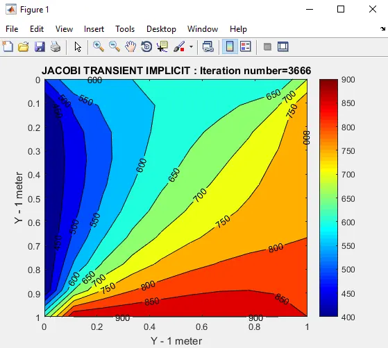

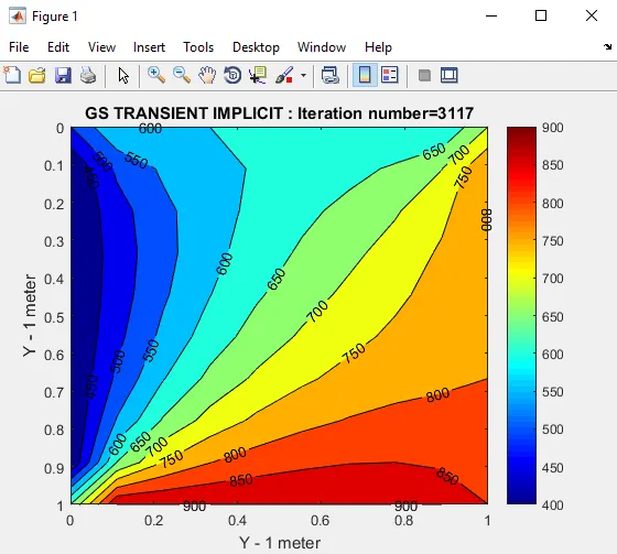
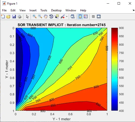
Discussion :

1.The code is structured in such a way that each code generates values for Jacobi , Gauss siedel & sor seperately but the code execution is same .
2.A square domain is chosen of dimension 1m .The domain is further discretised into a number of divisions along x & y axis and hence nx=ny=10
3.The tempratures on the walls of the domain is specified as boundary conditions ,the initial temprature to all the nodes apart from the boundary values is 300K.
Top Boundary = 600 K
Bottom Boundary = 900 K
Left Boundary = 400 K
Right Boundary = 800 K
4.Further the matrix's corner elements are average values of the adjacent elements and this is done to get better corner values while plotting the Temprature values .
5.A matrix copy for T is generated by equating T to Told which we will be using in the code for value updation.
6.'dx' & 'dy' are found out from the difference of the indeces of 'x' & 'y' respectively .
7.'K1, K2 & CFL' a constant is computed initially for further calculations by the program .
8.omega for SOR is declared,error & tolerance values are stated for the code to enter the while loop further in the code .
9. The while loop allows the code to run until the criteria error>tol.
10.The 2 'for loops' are for the code to calculate i & j positionn values in the matrix.
11.Jacobi , Gauss siedel or SOR gets executed for a given number iterations till the solution converges .
12.error is caluclated for the code to again enter the while loop until solution converges.
13.T values are updated into the Told matrix for use later in the for loop .
14.T_previous is the value of T from the previous time step .
16.The code uses contourf command to get a fully filled contour of the Temprature values in the graph .
17.''set(gca,'ydir','reverse')'' reverses the y axis for accurate output because Tbottom is 900K
18.colorbar gives the small vertical bar like scale for Temprature ranges generated in the code .
19.colormap(jet) is used to get distinct rgb colors in the graph .
20.clabel is used to label the temprature values on the graph in real time for every iteration .
21.title_text is used to display iteration values on the graph & also doubles as the code line uswed to write title of the graph .

--------------------------------------------------------------------------------------------------------------------------
The explicit method has the risk of generation of truncation error .
The implicit solution may be robust and versatile but the time taken is more than the rest of the methods
The time taken by Jacobi is more than Gauss siedel & Gauss Siedel takes more time than SOR .