Week 3 - Adiabatic Flame Temperature calculation
Aim :
- To understand the effect of equivalence ratio on AFT in a constant volume chamber .
- To view how the AFT changes for varying heat loss in a constant pressure chamber .
- To calculate AFT of alkanes,alkenes & alkynes in a 2 carbon chain hydrocarbon .
- To study how AFT changes for number of carbons in a hydrocarbon .
Background :
Air–fuel equivalence ratio (`lambda`) :
Air–fuel equivalence ratio, `lambda` (lambda), is the ratio of actual AFR to stoichiometry for a given mixture.
`lambda` = 1.0 is at stoichiometry,
rich mixtures `lambda` < 1.0,
and
lean mixtures `lambda` > 1.0.
There is a direct relationship between `lambda` and AFR. To calculate AFR from a given `lambda`, multiply the measured `lambda` by the stoichiometric AFR for that fuel. Alternatively, to recover `lambda` from an AFR, divide AFR by the stoichiometric AFR for that fuel. This last equation is often used as the definition of `lambda`:

Fuel air equivalence ratio `phi`:
The fuel–air equivalence ratio, `(phi)`, of a system is defined as the ratio of the fuel-to-oxidizer ratio to the stoichiometric fuel-to-oxidizer ratio. Mathematically,

where ‘m’ represents the mass, ‘n’ represents a number of moles, subscript ‘st’ stands for stoichiometric conditions.
The advantage of using equivalence ratio over fuel–oxidizer ratio is that it takes into account (and is therefore independent of) both mass and molar values for the fuel and the oxidizer.
Rich mixture : `phi>1`
Stoichiometric mix : `phi =1`
Lean mixture :`phi<1`
Adiabatic flame temprature :
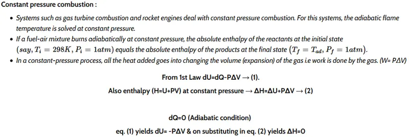
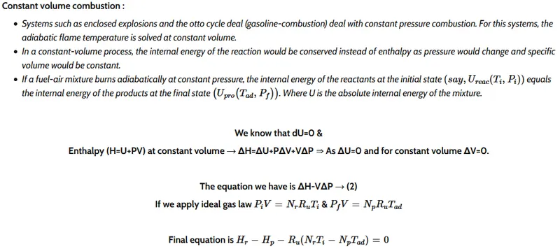
When a combustion reaction takes place energy is released to the combustion products. If no heat is lost in this process, the temperature of the combustion products is known as the "Adiabatic Flame Temperature."
Newton Raphson :
Let f(x) be a well-behaved function, and let ‘r’ be a root of the equation f(x) = 0. We start with an estimatex0ofr.From x0 , we produce an improved we hope estimate x1. From x1, we produce a new estimate x2.From x2, we produce a new estimate x3. We go on until we are `close enough' to ‘r’ or until it becomes clear that we are getting nowhere. The above general style of proceeding is called iterative . Of the many iterative root finding procedures, the Newton-Raphson method, with its com-bination of simplicity and power, is the most widely used.
Newton Raphson Iteration :
The Newton-Raphson Iteration Let ‘x0’ be a good estimate of ‘r’ and let r=x0+h. Since the true root is r , and h=r−x0, the number ‘h’ measures how far the estimate ‘x0’ is from the truth .Since his `small,' we can use the linear (tangent line) approximation to conclude that,
`0=f(r)=f(x_0+h)~~f(x_0)+hf_0'(x_0)`
and therefore, unless `f'_0(x_0)` is close to 0,
`h~~−f(x_0)/(f_0'(x_0))`
It follows that
`r=x_0+h~~x_0−f (x_0) / (f_0'(x_0))`
Our new improved estimate ‘x1’ of ‘r’ is therefore given by
`x_1=x_0−f(x_0)/(f_0'(x_0))`
The next estimate ’x2’ is obtained from ‘x1’ in exactly the same way as ‘x1’ was obtained from x0:
`x_2 = x_1 − f(x_1)/(f _0'(x_1))`
Continue in this way. If `x_n` is the current estimate, then the next estimate `x_(n+1)` is given by
`x_(n+1)=x_n−f(x_n)/(f_0’(x_n))`
NASA polynomial :
H = R*T*(a1 + a2 T /2 + a3 T^2 /3 + a4 T^3 /4 + a5 T^4 /5 + a6/T)
where a1, a2, a3, a4, a5 & a6 are the numerical coefficients supplied in NASA thermodynamic files. The first 7 numbers starting on the second line of each species entry (five of the second line and the first two of the third line) are the seven coefficients (a1 through a7, respectively) for the high-temperature range (above 1000 K, the upper boundary is specified on the first line of the species entry). The following seven numbers are the coefficients (a1 through a7, respectively) for the low-temperature range (below 1000 K, the lower boundary is specified on the first line of the species entry).
R = gas constant = 8.314 J/mol.K
The H denotes enthalpy which we will be using to find out the enthalpy of reactants and products .
NASA thermodynamic file : http://combustion.berkeley.edu/gri-mech/version30/files30/thermo30.dat
Challenge :
1. Adiabatic flame temperature variation with Equivalence ratio (In constant volume-chamber) :
General equation :
Let the amount of air be 'x' in the given reaction .
`CH_4 +x(O_2+3.76N_2) ->aCO_2 + bH_2O + c*3.76N_2`
The equivalence ratio is given by the following equation ,
`phi=((Fuel)/(Air))_(reaction)/((Fuel)/(Air))_(st oich)`
The fuel air mix value of a stoichiometric reaction is given below ,
`((Fuel)/(Air))_(st o ich)=1/2`
Let the amount of fuel in `((Fuel)/(Air))_(reaction)`be equal to 1
Substituting all the above in `phi`
`phi=((1)/(x))_(reaction)/((1)/(2))_(st oich)`
`phi=((1)/(x))*((2)/(1))`
`x=2/phi`
Substituting the value of 'x' in the general equation ,
`CH_4 + 2/phi(O_2+3.76N_2) ->aCO_2 + bH_2O + 2/phi*3.76N_2`
Stoichiometric : `phi`= 1
From the above equation ,
`CH_4 + 2/phi(O_2+3.76N_2) ->aCO_2 + bH_2O + 2/phi*3.76N_2`
Since `phi=1`
`CH_4 + 2(O_2+3.76N_2) -> CO_2 + 2H_2O + 2*3.76N_2`
Lean :`phi < 1`
`CH_4 + x(O_2+3.76N_2) ->aCO_2 + bH_2O + 3.76xN_2 + cO_2`
Considering `phi`the equivalence ratio
`CH_4 + 2/phi(O_2+3.76N_2) -> aCO_2 + bH_2O + 7.52/phiN_2 + cO_2`
Comparing the reactants side and the products side of the reaction
C : 1 = a
H : 4 = 2b `=> b=2`
O : `2/phi` = a + b/2 + c
Substituting a & b in 'O',
`2/phi=1+2/2+c`
`2/phi=2+c`
`c=2/phi-2`
Final equation becomes the following
`CH_4 + 2/phi(O_2+3.76N_2) -> CO_2 + 2H_2O +7.52/phiN_2 +( 2/phi– 2)O_2`
Rich :`phi>1`
`CH_4 + 2/phi(O_2+3.76N_2) -> aCO_2 + 2H_2O + 7.52/phiN_2 + dCO`
C : 1 = a+d
a = 1-d
H : 4 = 2b `=> b=2`
O : `2/phi=a+1+d/2`
Substituting a in above equation,
`2/phi=(1-d)+1+d/2`
`2/phi=2-d/2`
`d/2=2-2/phi`
`d=4-4/phi`
Substitute 'd' in 'a+d=1' to find out value of 'a'
`1=a+(4-4/phi)`
`a=1-(4-4/phi)`
`a=-3+4/phi`
Adiabatic flame temperature variation with respect to Alkane, Alkene, Alkyne :
`CH_4 + 2/phi(O_2+3.76N_2) -> (-3+4/phi)CO_2 + 2H_2O + 7.52/phiN_2 + (4-4/phi)CO`
Code :
https://drive.google.com/file/d/1apIMl1HTEOUrtTVjmnk7kQlLYZzhAYjh/view?usp=sharing
""" In this program we are going to calculate the AFT of methane at different equivalence ratios

CH4 + 2 (O2+3.76N2) = CO2 + 2 H2O + 7.52 N2

"""

import matplotlib.pyplot as plt
import math
import numpy as np
import cantera as ct

def h(T,coeffs): # within the parenthesis beside 'h' is the inputs required for the function
	"""
	Function to evaluate enthalpy
	"""
	R=8.314
	a1=coeffs[0]
	a2=coeffs[1]
	a3=coeffs[2]
	a4=coeffs[3]
	a5=coeffs[4]
	a6=coeffs[5]

	return (a1+a2*T/2+a3*pow(T,2)/3+a4*pow(T,3)/4+a5*pow(T,4)/5+a6/T)*R*T

ch4_coeffs_l=[5.14987613E+00,-1.36709788E-02,4.91800599E-05,-4.84743026E-08,1.66693956E-11,1.02466476E+04,-4.64130376E+00]
o2_coeffs_l=[3.78245636E+00,-2.99673416E-03,9.84730201E-06,-9.68129509E-09,3.24372837E-12,-1.06394356E+03,3.65767573E+00]
o2_coeffs_h=[3.28253784E+00,1.48308754E-03,-7.57966669E-07,2.09470555E-10,-2.16717794E-14,-1.08845772E+03,5.45323129E+00]
n2_coeffs_h=[0.02926640E+02,0.14879768E-02,-0.05684760E-05,0.10097038E-09,-0.06753351E-13,-0.09227977E+04,0.05980528E+02]
n2_coeffs_l=[0.03298677E+02,0.14082404E-02,-0.03963222E-04,0.05641515E-07,-0.02444854E-10,-0.10208999E+04,0.03950372E+02]
co2_coeffs_h=[3.85746029E+00,4.41437026E-03,-2.21481404E-06,5.23490188E-10,-4.72084164E-14,-4.87591660E+04,2.27163806E+00]
co_coeffs_h=[2.71518561E+00,2.06252743E-03,-9.98825771E-07,2.30053008E-10,-2.03647716E-14,-1.41518724E+04,7.81868772E+00]
h2o_coeffs_h=[3.03399249E+00,2.17691804E-03,-1.64072518E-07,-9.70419870E-11,1.68200992E-14,-3.00042971E+04,4.96677010E+00]


def f(T,phi):

	R=8.314

	""" Function that represents the root finding problem """

	h_co2_p=h(T,co2_coeffs_h)
	h_n2_p=h(T,n2_coeffs_h)
	h_h2o_p=h(T,h2o_coeffs_h)
	h_o2_p=h(T,o2_coeffs_h)
	h_co_p=h(T,co_coeffs_h)

	Tstd=273.15
	h_ch4_r=h(Tstd,ch4_coeffs_l)
	h_o2_r=h(Tstd,o2_coeffs_l)
	h_n2_r=h(Tstd,n2_coeffs_l)

	H_reactants=h_ch4_r+2*h_o2_r+2*3.76*h_n2_r
	print(H_reactants)
	n_r = (1 + (2/phi) + (2/phi)*3.76)*Tstd*R

	if phi<=1:
		# CH_4 + 2/phi(O_2+3.76N_2) = CO_2 + 2H_2O +7.52/phiN_2 +( 2/phi– 2)O_2
		#H_reactants_rich-H_products_rich-R*(n_r_3*Tstd-n_p_3*T)
		H_products=h_co2_p+2*h_h2o_p+(7.52/phi)*h_n2_p+((2/phi)-2)*h_o2_p
		print(H_products)
		n_p = (1 + 2 + (7.52/phi) + ((2/phi)-2))*R*T
	elif phi>1:
		# CH_4 + 2/phi(O_2+3.76N_2)=(4/phi– 3) CO_2 + 2H_2O + 7.52/phi N_2 +(4-(4/phi)) CO
		H_products=((4/phi)-3)*h_co2_p+2*h_h2o_p+(7.52/phi)*h_n2_p+(4-(4/phi))*h_co_p
		print(H_products)
		n_p = (((4/phi)-3)+2+(7.52/phi)+(4-(4/phi)))*R*T

	return H_reactants-H_products-(n_p-n_r)

def fprime(T,phi):
	""" numerical derivative = forward differencing """
	return(f(T+1e-6,phi)-f(T,phi))/1e-6

T_guess = 1500
tol = 1e-3
alpha = 0.2

phi=np.linspace(0.1,2,39)
print(phi)

T_aft=[]

for i in range(0,len(phi)):
	while(abs(f(T_guess,phi[i])) > tol):
		T_guess = T_guess - alpha*(f(T_guess,phi[i])/fprime(T_guess,phi[i]))
	T_aft.append(T_guess)

print(T_aft)
plt.plot(phi,T_aft,label='Python',color='blue')
plt.grid('on')

"""
Canrtra program for AFT at different equivalence ratios

"""

T_cantera=[]

for j in range(0,len(phi)):
	gas = ct.Solution('gri30.xml')
	gas.TPX=298.15,101325,{'CH4':1,'O2':2/phi[j],'N2':(2*3.76)/phi[j]}
	gas.equilibrate('HP','auto')
	T_cantera.append(gas.T)


plt.plot(phi,T_cantera,label='Cantera')
plt.title('Methane : Equivalence ratio vs AFT')
plt.xlabel('Equivalence ratio [Phi]',)
plt.ylabel('Adiabatic flame temprature [K]')
plt.legend()
plt.show()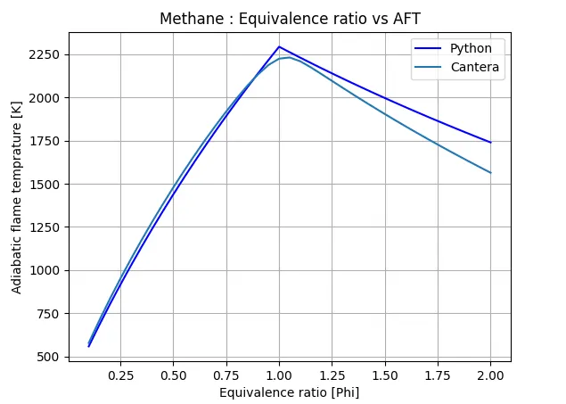
Observation :
- Here we can see clearly that the code from python is plotted alongside the results obtained from Cantera ,this shows that the logic used in the python code is acceptble .
- We can also see that the cantera plot of the AFT beyond `phi=1`shows a lesser value in temprature than that of the python because Cantera considers a lot more species than what we have considered and the enthalpy gets distributed to those many products and produces an overall lower value in AFT .
2. Adiabatic flame temperature variation with Heat loss (In constant pressure-chamber) :
Code :
https://drive.google.com/file/d/1H8l1E4KBoSjokH-xeWvCX_Gx6S0A0kX5/view?usp=sharing
""" Adiabatic flame temperature variation with Heat loss (In constant pressure-chamber)

CH4 + 2 (O2 + 3.76N2) = CO2 + 2 H2O + 7.52 N2

"""

import matplotlib.pyplot as plt
import math
import numpy as np


def h(T,coeffs): # within the parenthesis (beside 'h',whereas h is name of function) is the inputs required for the function
	"""Function to evaluate enthalpy
	"""
	R=8.314
	a1=coeffs[0]
	a2=coeffs[1]
	a3=coeffs[2]
	a4=coeffs[3]
	a5=coeffs[4]
	a6=coeffs[5]

	return (a1+a2*T/2+a3*pow(T,2)/3+a4*pow(T,3)/4+a5*pow(T,4)/5+a6/T)*R*T

ch4_coeffs_l=[5.14987613E+00,-1.36709788E-02,4.91800599E-05,-4.84743026E-08,1.66693956E-11,-1.02466476E+04,-4.64130376E+00]
o2_coeffs_l=[3.78245636E+00,-2.99673416E-03,9.84730201E-06,-9.68129509E-09,3.24372837E-12,-1.06394356E+03,3.65767573E+00]
n2_coeffs_h=[0.02926640E+02,0.14879768E-02,-0.05684760E-05,0.10097038E-09,-0.06753351E-13,-0.09227977E+04,0.05980528E+02]
n2_coeffs_l=[0.03298677E+02,0.14082404E-02,-0.03963222E-04,0.05641515E-07,-0.02444854E-10,-0.10208999E+04,0.03950372E+02]
co2_coeffs_h=[3.85746029E+00,4.41437026E-03,-2.21481404E-06,5.23490188E-10,-4.72084164E-14,-4.87591660E+04,2.27163806E+00]
h2o_coeffs_h=[3.03399249E+00,2.17691804E-03,-1.64072518E-07,-9.70419870E-11,1.68200992E-14,-3.00042971E+04,4.96677010E+00]

def f(T,Heat_loss,LHV):
	""" Function that represents the root finding problem """
	h_co2_p=h(T,co2_coeffs_h)
	h_n2_p=h(T,n2_coeffs_h)
	h_h2o_p=h(T,h2o_coeffs_h)

	H_products=h_co2_p+2*h_h2o_p+7.52*h_n2_p
	print(H_products)

	Tstd=273.15
	h_ch4_r=h(Tstd,ch4_coeffs_l)
	h_o2_r=h(Tstd,o2_coeffs_l)
	h_n2_r=h(Tstd,n2_coeffs_l)

	H_reactants=h_ch4_r+2*h_o2_r+2*3.76*h_n2_r
	print(H_reactants)

	return H_products-H_reactants+Heat_loss*LHV

def fprime(T,Heat_loss,LHV):
	""" numerical derivative = forward differencing """

	return(f(T+1e-6,Heat_loss,LHV)-f(T,Heat_loss,LHV))/1e-6

T_guess=1500
tol=1e-3
ct=0
alpha = 0.2

LHV=802340 #kj/mol &  55 MJ/kg
print(LHV)

Heat_loss=np.linspace(0,1,41)
print(Heat_loss)

T_aft=[]

for i in range(0,len(Heat_loss)):
	while(abs(f(T_guess,Heat_loss[i],LHV))>tol):
		T_guess=T_guess-alpha*((f(T_guess,Heat_loss[i],LHV)/fprime(T_guess,Heat_loss[i],LHV)))
	T_aft.append(T_guess)

print(T_aft)

""" FOR LABEL ON PLOT OF ATF AT 0.35*H_loss & plotting a graph """

a=np.searchsorted(Heat_loss,0.35) # finds 0.35 from linspace of H_loss
b=round(Heat_loss[a],3) # rounds off to the thrid decimal & Calls value of H_loss at index [a].
print(a)
print(b)

c=round(T_aft[a],3) # Calls the 'a'th AFT value corresponding to the 0.35*H_loss on X axis
print(c)

plt.plot(Heat_loss,T_aft,color='red') # plots the aft vs heat loss graph
plt.plot(b,c,'*',color='black') # used to mark 0.35*H_loss

label = f"(Heatloss = {b}, aft = {c} K)" # used as a label for the marked point on plot
plt.annotate(label,(b,c)) # shows where the point is located and calls the label to that location

plt.xlabel('Heat loss')
plt.ylabel('Adiabatic flame temprature [K]')
plt.title('AFT vs Heat loss')
plt.show()
Output :
Observation :
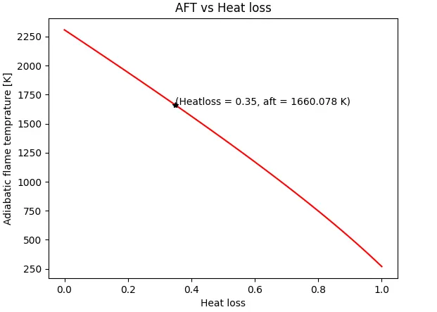
- AFT at 0.35 heat loss is 1660.078 K .
- The heat loss factor at 0 simply means AFT at stoichiometric condition of methane .
3. Adiabatic flame temperature variation with respect to Alkane, Alkene, Alkyne :
Ethane :
`C_2H_6+ar(O_2+3.76N_2) ->aCO_2+bH_2O+cN_2`
C : 2=a
H : 6=2b
O : ar=a+b/2
So, a=2 , b=3 , ar=2+3/2=3.5
`C_2H_6+ar(O_2+3.76N_2) ->2CO_2+3H_2O+(3.5)3.76N_2`
Ethene :
`C_2H_4+ar(O_2+3.76N_2) ->aCO_2+bH_2O+cN_2`
C : 2=a
H : 4=2b
O : ar=a+b/2
So, a=2 , b=2 , ar=2+2/2=3
`C_2H_6+ar(O_2+3.76N_2) ->2CO_2+2H_2O+(3)*3.76N_2`
Etheye :
`C_2H_2+ar(O_2+3.76N_2) ->aCO_2+bH_2O+cN_2`
C : 2=a
H : 2=2b
O : ar=a+b/2
So, a=2 , b=1 , ar=2+1/2=2.5
`C_2H_6+2.5(O_2+3.76N_2) ->2CO_2+H_2O+(2.5)*3.76N_2`
Code :
https://drive.google.com/file/d/1UZXCmjZG1xNheTON353AgBuGaOo7rlET/view?usp=sharing
""" Alkane ,Alkene ,Alkyne of 2 carbon atom chain vs AFT

C2H6 + 3.5 (O2 + 3.76N2) = 2*CO2 + 3*H2O + 3.5*3.76 N2
C2H4 + 3 (O2 + 3.76N2) = 2CO2 + 2 H2O + 3*3.76 N2
C2H2 + 2.5 (O2 + 3.76N2) = 2 CO2 +  H2O + 2.5*3.76 N2

"""
import matplotlib.pyplot as plt
import math

def h(T,coeffs): # within the parenthesis beside 'h' is the inputs required for the function
	"""Function to evaluate enthalpy
	"""
	R=8.314
	a1=coeffs[0]
	a2=coeffs[1]
	a3=coeffs[2]
	a4=coeffs[3]
	a5=coeffs[4]
	a6=coeffs[5]

	return (a1+a2*T/2+a3*pow(T,2)/3+a4*pow(T,3)/4+a5*pow(T,4)/5+a6/T)*R*T

c2h6_coeffs_l=[4.29142492E+00,-5.50154270E-03,5.99438288E-05,-7.08466285E-08,2.68685771E-11,-1.15222055E+04,2.66682316E+00]
c2h4_coeffs_l=[3.95920148E+00,-7.57052247E-03,5.70990292E-05,-6.91588753E-08,2.69884373E-11,5.08977593E+03,4.09733096E+00]
c2h2_coeffs_l=[8.08681094E-01,2.33615629E-02,-3.55171815E-05,2.80152437E-08,-8.50072974E-12,2.64289807E+04,1.39397051E+01]
o2_coeffs_l=[3.78245636E+00,-2.99673416E-03,9.84730201E-06,-9.68129509E-09,3.24372837E-12,-1.06394356E+03,3.65767573E+00]
n2_coeffs_h=[0.02926640E+02,0.14879768E-02,-0.05684760E-05,0.10097038E-09,-0.06753351E-13,-0.09227977E+04,0.05980528E+02]
n2_coeffs_l=[0.03298677E+02,0.14082404E-02,-0.03963222E-04,0.05641515E-07,-0.02444854E-10,-0.10208999E+04,0.03950372E+02]
co2_coeffs_h=[3.85746029E+00,4.41437026E-03,-2.21481404E-06,5.23490188E-10,-4.72084164E-14,-4.87591660E+04,2.27163806E+00]
h2o_coeffs_h=[3.03399249E+00,2.17691804E-03,-1.64072518E-07,-9.70419870E-11,1.68200992E-14,-3.00042971E+04,4.96677010E+00]

def f(T,H):
	""" Function that represents the root finding problem 	"""

	Tstd=273.15

	"""C2H6 + 3.5 (O2 + 3.76N2) = 2*CO2 + 3*H2O + 3.5*3.76 N2
	C2H4 + 3 (O2 + 3.76N2) = 2CO2 + 2 H2O + 3*3.76 N2
	C2H2 + 2.5 (O2 + 3.76N2) = 2 CO2 +  H2O + 2.5*3.76 N2"""


	h_c2h6_r=h(Tstd,c2h6_coeffs_l)
	h_c2h4_r=h(Tstd,c2h4_coeffs_l)
	h_c2h2_r=h(Tstd,c2h2_coeffs_l)

	h_o2_r=h(Tstd,o2_coeffs_l)
	h_n2_r=h(Tstd,n2_coeffs_l)

	h_co2_p=h(T,co2_coeffs_h)
	h_n2_p=h(T,n2_coeffs_h)
	h_h2o_p=h(T,h2o_coeffs_h)

	if H==1:
	# ETHANE
	# C2H6 + 3.5 (O2 + 3.76N2) = 2*CO2 + 3*H2O + 3.5*3.76 N2
		H_reactants=h_c2h6_r+3.5*(h_o2_r+3.76*h_n2_r)
		H_products=2*h_co2_p+3*h_h2o_p+3.5*3.76*h_n2_p
		return H_products-H_reactants

	elif H==2:
	# ETHENE
	#C2H4 + 3 (O2 + 3.76N2) = 2CO2 + 2 H2O + 3*3.76 N2
		H_reactants=h_c2h4_r+3*(h_o2_r+3.76*h_n2_r)
		H_products=2*h_co2_p+2*h_h2o_p+3*3.76*h_n2_p
		return H_products-H_reactants

	else:
	# ETHYNE
	# C2H2 + 2.5 (O2 + 3.76N2) = 2 CO2 +  H2O + 2.5*3.76 N2
		H_reactants=h_c2h2_r+2.5*(h_o2_r+3.76*h_n2_r)
		H_products=2*h_co2_p+h_h2o_p+2.5*3.76*h_n2_p
		return H_products-H_reactants

def fprime(T,H):
	""" numerical derivative = forward differencing """
	if H==1:
		return(f(T+1e-6,H)-f(T,H))/1e-6

	elif H==2:
		return(f(T+1e-6,H)-f(T,H))/1e-6

	else:
		return(f(T+1e-6,H)-f(T,H))/1e-6

T_guess=1500
tol=1e-3
ct=0
alpha = 0.2

H=[1,2,3] # condition for number of carbon atoms
i=[1,2,3]

T_aft=[]

for i in range(0,len(H)):
	while abs(f(T_guess,H[i])) > tol:
		T_guess=T_guess-alpha*((f(T_guess,H[i])/fprime(T_guess,H[i])))
		#ct=ct+1
	T_aft.append(T_guess)

print(T_aft)

plt.plot('C2H6',T_aft[0],'v',color='cornflowerblue')
plt.plot('C2H4',T_aft[1],'v',color='cornflowerblue')
plt.plot('C2H2',T_aft[2],'v',label='Python',color='cornflowerblue')

""" Cantera code """

import cantera as ct

"""

C2H6 + 3.5 (O2 + 3.76N2) = 2*CO2 + 3*H2O + 3.5*3.76 N2
C2H4 + 3 (O2 + 3.76N2) = 2CO2 + 2 H2O + 3*3.76 N2
C2H2 + 2.5 (O2 + 3.76N2) = 2 CO2 +  H2O + 2.5*3.76 N2

"""

gas = ct.Solution('gri30.xml')
gas.TPX=298.15,101325,{'C2H6':1,'O2':3.5,'N2':13.16}
gas.equilibrate('HP','auto')
ethane=gas.T
print(gas.T)

gas.TPX=298.15,101325,{'C2H4':1,'O2':3,'N2':11.28}
gas.equilibrate('HP','auto')
ethene=gas.T
print(gas.T)

gas.TPX=298.15,101325,{'C2H2':1,'O2':2.5,'N2':9.4}
gas.equilibrate('HP','auto')
ethyne=gas.T
print(gas.T)

T_cant=[ethane,ethene,ethyne]

plt.plot('C2H6',T_cant[0],'o',color='darksalmon')
plt.plot('C2H4',T_cant[1],'o',color='darksalmon')
plt.plot('C2H2',T_cant[2],'o',label='Python',color='darksalmon')
plt.legend()
plt.title('Ethane ,Ethene ,Ethyne (of 2 carbon atom chain) vs AFT')
plt.xlabel('Type of Hydrocarbon')
plt.ylabel('Adiabatic flame temprature [K]')

plt.show()
Output :
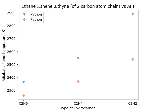
Observation :
- With a decreasing trend in ratio of carbon to hydrogen atoms in a hydrocarbon ,the AFT increases significantly .
Since we have considered the stoichiometric reactions of the hydrocarbons we can draw a comparison between carbon and hydrogen atoms and it's effect on AFT .
In ethane : Carbon to hydrogen ratio is 1:3 = 0.333In ethane : Carbon to hydrogen ratio is 1:2 = 0.5In ethane : Carbon to hydrogen ratio is 1:1 = 1
As the value of carbon to hydrogen ratio increases the AFT attained by that hydrocarbon increases on combustion . - Since cantera takes many products of combustion into account it generates a lesser value of AFT when compared to the python code .
4. Adiabatic flame temperature variation with respect to a number of Carbon atom chains :
Carbon atoms (from 1 to 3)
Methane :
`CH_4+ar(O_2+3.76N_2) ->aCO_2+bH_2O+cN_2`
C : 1=a
H : 4=2b
O : ar=a+b/2
So, a=1 , b=2 , ar=1+2/2 = 2
`CH_4+2(O_2+3.76N_2) ->CO_2+2H_2O+2*3.76N_2`
Ethane :
`C_2H_6+ar(O_2+3.76N_2) ->aCO_2+bH_2O+cN_2`
C : 2=a
H : 6=2b
O : ar=a+b/2
So, a=2 , b=3 , ar=2+3/2=3.5
`C_2H_6+3.5(O_2+3.76N_2) ->2CO_2+3H_2O+(3.5)3.76N_2`
Propane :
`C_3H_8+ar(O_2+3.76N_2) ->aCO_2+bH_2O+cN_2`
C : 3=a
H : 8=2b
O : ar=a+b/2
So, a=3 , b=4 , ar=3+4/2 = 5
`C_3H_8+5(O_2+3.76N_2) ->3CO_2+4H_2O+(5)*3.76N_2`
Code :
https://drive.google.com/file/d/1q4SLwWY1XyNlmDvkWlns4pn93hPUYVZ4/view?usp=sharing
""" In this program we are going to calculate the AFT of Methane, Ethane & Propane


CH4 + 2 (O2 + 3.76N2) = CO2 + 2 H2O + 7.52 N2
C2H6 + 3.5 (O2 + 3.76N2) = 2CO2 + 3H2O + 13.16 N2
C3H8 + 5 (O2 + 3.76N2) = 3CO2 + 4H2O + 18.8 N2


"""

import matplotlib.pyplot as plt
import math

C=[1,2,3] # condition for number of carbon atoms
i=[1,2,3]

def h(T,coeffs): # within the parenthesis beside 'h' is the inputs required for the function
	"""

	Function to evaluate enthalpy

	"""
	R=8.314
	a1=coeffs[0]
	a2=coeffs[1]
	a3=coeffs[2]
	a4=coeffs[3]
	a5=coeffs[4]
	a6=coeffs[5]

	return (a1+a2*T/2+a3*pow(T,2)/3+a4*pow(T,3)/4+a5*pow(T,4)/5+a6/T)*R*T

ch4_coeffs_l=[5.14987613E+00,-1.36709788E-02,4.91800599E-05,-4.84743026E-08,1.66693956E-11,-1.02466476E+04,-4.64130376E+00]
c2h6_coeffs_l=[4.29142492E+00,-5.50154270E-03,5.99438288E-05,-7.08466285E-08,2.68685771E-11,-1.15222055E+04,2.66682316E+00]
c3h8_coeffs_l=[0.93355381E+00,0.26424579E-01,0.61059727E-05,-0.21977499E-07,0.95149253E-11,-0.13958520E+05,0.19201691E+02]
o2_coeffs_l=[3.78245636E+00,-2.99673416E-03,9.84730201E-06,-9.68129509E-09,3.24372837E-12,-1.06394356E+03,3.65767573E+00]
n2_coeffs_h=[0.02926640E+02,0.14879768E-02,-0.05684760E-05,0.10097038E-09,-0.06753351E-13,-0.09227977E+04,0.05980528E+02]
n2_coeffs_l=[0.03298677E+02,0.14082404E-02,-0.03963222E-04,0.05641515E-07,-0.02444854E-10,-0.10208999E+04,0.03950372E+02]
co2_coeffs_h=[3.85746029E+00,4.41437026E-03,-2.21481404E-06,5.23490188E-10,-4.72084164E-14,-4.87591660E+04,2.27163806E+00]
h2o_coeffs_h=[3.03399249E+00,2.17691804E-03,-1.64072518E-07,-9.70419870E-11,1.68200992E-14,-3.00042971E+04,4.96677010E+00]

def f(T,C):
	""" Function that represents the root finding problem """

	Tstd=273.15

	"""CH4 + 2 (O2 + 3.76N2) = CO2 + 2 H2O + 7.52 N2
	C2H6 + 3.5 (O2 + 3.76N2) = 2CO2 + 3H2O + 13.1 N2
	C3H8 + 5 (O2 + 3.76N2) = 3CO2 + 4H2O + 18.8 N2"""

	h_ch4_r=h(Tstd,ch4_coeffs_l)
	h_c2h6_r=h(Tstd,c2h6_coeffs_l)
	h_c3h8_r=h(Tstd,c3h8_coeffs_l)

	h_o2_r=h(Tstd,o2_coeffs_l)
	h_n2_r=h(Tstd,n2_coeffs_l)

	h_co2_p=h(T,co2_coeffs_h)
	h_n2_p=h(T,n2_coeffs_h)
	h_h2o_p=h(T,h2o_coeffs_h)

	if C==1:
		H_reactants=h_ch4_r+2*(h_o2_r+3.76*h_n2_r)
		H_products=h_co2_p+2*h_h2o_p+2*3.76*h_n2_p
		return H_products-H_reactants

	elif C==2:
		H_reactants=h_c2h6_r+3.5*(h_o2_r+3.76*h_n2_r)
		H_products=2*h_co2_p+3*h_h2o_p+3.5*3.76*h_n2_p
		return H_products-H_reactants

	else:
		H_reactants=h_c3h8_r+5*(h_o2_r+3.76*h_n2_r)
		H_products=3*h_co2_p+4*h_h2o_p+5*3.76*h_n2_p
		return H_products-H_reactants

def fprime(T,C):
	""" numerical derivative = forward differencing """
	if C==1:
		return(f(T+1e-6,C)-f(T,C))/1e-6

	elif C==2:
		return(f(T+1e-6,C)-f(T,C))/1e-6

	else:
		return(f(T+1e-6,C)-f(T,C))/1e-6

T_guess=1500
tol=1e-3
ct=0
alpha = 0.2
T_aft=[]

for i in range(0,len(C)):
	while abs(f(T_guess,C[i])) > tol:
		T_guess=T_guess-alpha*((f(T_guess,C[i])/fprime(T_guess,C[i])))
		#ct=ct+1
	T_aft.append(T_guess)

print(T_aft)
print('aft for methane,ethane & propane ='+ str(T_aft))
plt.plot('CH4',T_aft[0],'v',color='cornflowerblue')
plt.plot('C2H6',T_aft[1],'v',color='cornflowerblue')
plt.plot('C3H8',T_aft[2],'v',label='Python',color='cornflowerblue')

""" Cantera code """

import cantera as ct

"""

CH4 + 2 (O2 + 3.76N2) = CO2 + 2 H2O + 7.52 N2
C2H6 + 3.5 (O2 + 3.76N2) = 2CO2 + 3H2O + 13.16 N2
C3H8 + 5 (O2 + 3.76N2) = 3CO2 + 4H2O + 18.8 N2

"""

gas = ct.Solution('gri30.xml')
gas.TPX=298.15,101325,{'CH4':1,'O2':2,'N2':7.52}
gas.equilibrate('HP','auto')
methane=gas.T
print(gas.T)

gas.TPX=298.15,101325,{'C2H6':1,'O2':3.5,'N2':13.16}
gas.equilibrate('HP','auto')
ethane=gas.T
print(gas.T)

gas.TPX=298.15,101325,{'C3H8':1,'O2':5,'N2':18.8}
gas.equilibrate('HP','auto')
propane=gas.T
print(gas.T)

T_cant=[methane,ethane,propane]

plt.plot('CH4',T_cant[0],'o',color='darksalmon')
plt.plot('C2H6',T_cant[1],'o',color='darksalmon')
plt.plot('C3H8',T_cant[2],'o',label='Cantera',color='darksalmon')
plt.title('Methane, Ethane & Propane vs AFT')
plt.xlabel('Type of Hydrocarbon')
plt.ylabel('Adiabatic flame temprature [K]')
plt.legend()

plt.show()
Output :
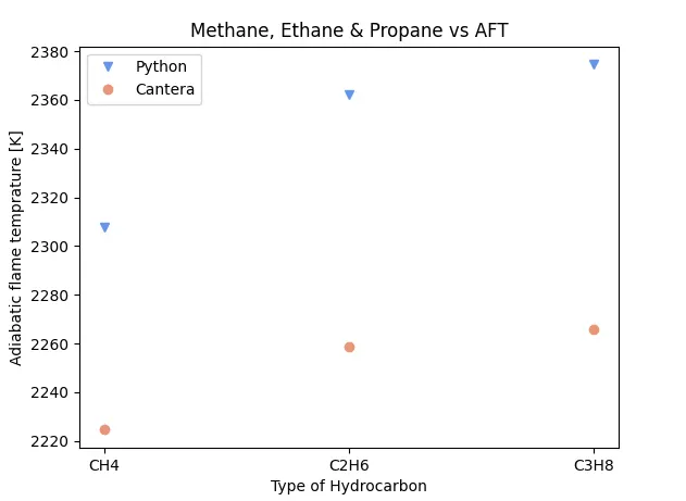
Observation :
- As the number of carbon atoms in the hydrocarbon increases the AFT of that hydrocarbon increases dramatically .
Since we have considered the stoichiometric reactions of the hydrocarbons we can draw a comparison between carbon and hydrogen atoms and it's effect on AFT.In methane : Carbon to Hydrogen ratio is 1:4 = 0.25In ethane : Carbon to Hydrogen ratio is 2:6 = 0.333In propane : Carbon to Hydrogen ratio is 3:8 = 0.375As the value of carbon to hydrogen ratio increases the AFT attained by that hydrocarbon increases on combustion . - Since cantera takes many products of combustion into account it generates a lesser value of AFT when compared to the python code .