Supervised Learning - Prediction Week 3 Challenge

1. Perform Gradient Descent in Python with any loss function

Gradient descent (GD) is an iterative first-order optimisation algorithm used to find a local minimum/maximum of a given function. This method is commonly used in machine learning (ML) and deep learning(DL) to minimise a cost/loss function (e.g. in a linear regression). Due to its importance and ease of implementation, this algorithm is usually taught at the beginning of almost all machine learning courses.
However, its use is not limited to ML/DL only, it’s being widely used also in areas like:

• Control engineering (robotics, chemical, etc.)
• Computer games
• Mechanical engineering
  
  

That’s why today we will get a deep dive into the math, implementation and behaviour of first-order gradient descent algorithm. We will navigate the custom (cost) function directly to find its minimum, so there will be no underlying data like in typical ML tutorials — we will be more flexible in terms of a function’s shape.
This method was proposed before the era of modern computers and there was an intensive development meantime which led to numerous improved versions of it but in this article, we’re going to use a basic/vanilla gradient descent implemented in Python.

Gradient descent:

It may help to review some concepts from linear regression. You may recall the following formula for the slope of a line, which is y = mx + b, where m represents the slope and b is the intercept on the y-axis.

You may also recall plotting a scatterplot in statistics and finding the line of best fit, which required calculating the error between the actual output and the predicted output (y-hat) using the mean squared error formula. The gradient descent algorithm behaves similarly, but it is based on a convex function, such as the one below:

The starting point is just an arbitrary point for us to evaluate the performance. From that starting point, we will find the derivative (or slope), and from there, we can use a tangent line to observe the steepness of the slope. The slope will inform the updates to the parameters—i.e. the weights and bias. The slope at the starting point will be steeper, but as new parameters are generated, the steepness should gradually reduce until it reaches the lowest point on the curve, known as the point of convergence.

Similar to finding the line of best fit in linear regression, the goal of gradient descent is to minimize the cost function, or the error between predicted and actual y. In order to do this, it requires two data points—a direction and a learning rate. These factors determine the partial derivative calculations of future iterations, allowing it to gradually arrive at the local or global minimum (i.e. point of convergence). More detail on these components can be found below:

• Learning rate (also referred to as step size or the alpha) is the size of the steps that are taken to reach the minimum. This is typically a small value, and it is evaluated and updated based on the behavior of the cost function. High learning rates result in larger steps but risks overshooting the minimum. Conversely, a low learning rate has small step sizes. While it has the advantage of more precision, the number of iterations compromises overall efficiency as this takes more time and computations to reach the minimum.

Procedure of gradient descent:

The procedure starts off with initial values for the coefficient or coefficients for the function. These could be 0.0 or a small random value.
coefficient = 0.0

The cost of the coefficients is evaluated by plugging them into the function and calculating the cost.

cost = f(coefficient)
or
cost = evaluate(f(coefficient))

The derivative of the cost is calculated. The derivative is a concept from calculus and refers to the slope of the function at a given point. We need to know the slope so that we know the direction (sign) to move the coefficient values in order to get a lower cost on the next iteration.

delta = derivative(cost)

Now that we know from the derivative which direction is downhill, we can now update the coefficient values. A learning rate parameter (alpha) must be specified that controls how much the coefficients can change on each update.

coefficient = coefficient – (alpha * delta)

This process is repeated until the cost of the coefficients (cost) is 0.0 or close enough to zero to be good enough.

You can see how simple gradient descent is. It does require you to know the gradient of your cost function or the function you are optimizing, but besides that, it’s very straightforward. Next we will see how we can use this in machine learning algorithms.

Derivation of the differential of the loss function:

`E = 1/n*sum_(i=0)^n ((y_i)-(mx_i+c))^2`

`(dE)/(dm) = 1/n*sum_(i=0)^n*(d)/(dm)(y_i-(mx_i+c)^2)`

`(dE)/(dm) = 1/n*sum_(i=0)^n (d/(dm))((y_i)^2+(mx_i+c)^2-2y_i(mx_i+c))`

`(dE)/(dm) = 1/n*sum_(i=0)^n (d/(dm))((y_i)^2+(mx_i)^2+c^2+2mx_ic-2y_imx_i+2y_ic)`

`(dE)/(dm) = 1/n*sum_(i=0)^n[(dy_i^2)/(dm)+(d(mx_i)^2)/(dm)+(d(c)^2)/(dm)+(d(2mcx_i))/(dm)-(d(2my_ix_i))/(dm)-(d(2y_ic))/(dm)]`

Here, `[(d(2y_ic))/(dm),(d(c)^2)/(dm),(dy_i^2)/(dm)]=0`

`(dE)/(dm) = 1/n*sum_(i=0)^n[(d(mx_i)^2)/(dm)+(d(2mcx_i))/(dm)-(d(2my_ix_i))/(dm)]`

Applying product rule to the first term,

`(d(mx_i)^2)/(dm)=(d(m)^2)/(dm)*(x_i)^2+(d(x_i)^2)/(dm)*(m)^2 = 2m(x_i)^2`

`(dE)/(dm) = 1/n*sum_(i=0)^n[2mx_i^2+2x_ic-2y_ix_i]`

`(dE)/(dm) = 2/n*sum_(i=0)^n[mx_i^2+x_ic-y_ix_i]`

`(dE)/(dm) = -2/n*sum_(i=0)^n(x_i)[y_i-(mx_i+c)]`

`E = 1/n*sum_(i=0)^n ((y_i)-(mx_i+c))^2`

`(dE)/(dc) = 1/n*sum_(i=0)^n ((y_i)-(mx_i+c))^2`

`(dE)/(dc) = 1/n*sum_(i=0)^n (d/(dc))((y_i)^2+(mx_i+c)^2-2y_i(mx_i+c))`

`(dE)/(dc) = [1/n]*sum_(i=0)^n (d/(dc))((y_i)^2+(mx_i)^2+c^2+2mx_ic-2y_imx_i-2y_ic)`

`(dE)/(dc) = [1/n]*sum_(i=0)^n (((d(y_i)^2)/(dc))+((d(mx_i)^2)/(dc))+((d(c^2))/(dc))+((d(2mx_ic))/(dc))-((d(2y_imx_i))/(dc))-((d(2y_ic))/(dc)))`

Here,

`[(d(2my_ix_i))/(dc),(d(mx_i)^2)/(dc),(dy_i^2)/(dc)]=0`

`(dE)/(dc) = [1/n]*sum_(i=0)^n (((d(c^2))/(dc))+((d(2mx_ic))/(dc))-((d(2y_ic))/(dc)))`

`(dE)/(dc) = [1/n]*sum_(i=0)^n (2c+2mx_i-2y_i)`

`(dE)/(dc) = [-2/n]*sum_(i=0)^n (-c-mx_i+y_i)`

`(dE)/(dc) = [-2/n]*sum_(i=0)^n (y_i-(mx_i+c))`

Univariate linear regression:

Dataset: https://drive.google.com/file/d/1NdUkGUaERcltgdGPw_41YxhwvVBzpah9/view?usp=sharing

import numpy as np
import pandas as pd
import matplotlib.pyplot as plt
from scipy.sparse.construct import rand

#plt.rcParams['figure.figsize'] = (12.0, 9.0)
df = pd.read_csv('dataset_one.csv')
print(df)
print(df.shape)

x = df.iloc[:, 0]
y = df.iloc[:, 1]
plt.scatter(x, y)
plt.xlabel('X')
plt.ylabel('Y')
plt.legend(['Datapoints'])
plt.show()

m = 0
c = 0
L = 0.0001  # Learning Rate
iter = 100  # Number of iterations to perform gradient descent
n = len(x) # Number of elements in X
print(n)
# def simple_linear_regression():

m_empty = []
c_empty = []

for j in range(0, 100):
    for i in range(0, len(x)):

        y_pred = m*x + c
        #print(y_pred)

        D_m = -(2/n) * np.sum(x * (y - y_pred))
        #print('dm = ', D_m)
        D_c = -(2/n) * np.sum(y - y_pred)
        #print(D_c)

        m = m - L* D_m
        c = c - L* D_c

        # syntax for append: list_name.append(item)
        m_empty.append(m)
        c_empty.append(c)

print('Values of m and c = ', m,c)

y_pred = m*x + c

plt.scatter(x, y)
plt.plot([min(x), max(x)], [min(y_pred), max(y_pred)], color='red')  # regression line
plt.legend(['Datapoints', 'Linear regression line'])
plt.xlabel('X')
plt.ylabel('Y')
plt.show()

# verification using sklearn
from sklearn.model_selection import train_test_split
from sklearn.linear_model import LinearRegression
X_train, X_test, y_train, y_test = train_test_split(x, y, test_size=0.2, random_state=0)
regressor = LinearRegression()
regressor.fit(X_train.values.reshape(-1, 1), y_train)
y_predicted = regressor.predict(X_test.values.reshape(-1, 1))
df1 = pd.DataFrame({'Actual': y_test, 'Predicted': y_predicted})
print(df1)

error = abs(y_test - y_predicted)
print('Error = ', error)
f = np.linspace(0, len(error))

plt.hist(error, bins=18, color=(0.1, 0.1, 0.1, 0.1), edgecolor='blue')
plt.ylabel('Error Magnitude')
plt.show()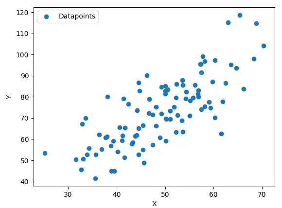

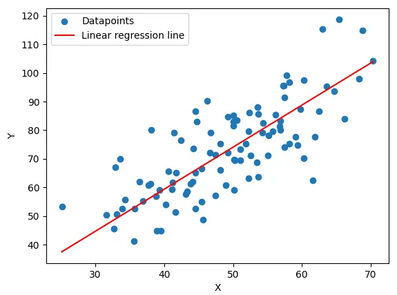
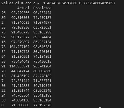
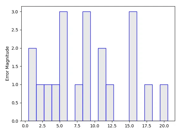
From the below comparison we can see the error.

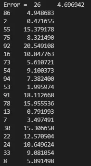
Data for multivariate linear regression:

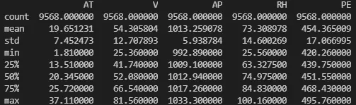
Since the mean is not equal to 0 and the standard deviation is not equal to 1, normalization must be used intstead of standardization.

Multivariate regression using normalization:

Dataset: https://drive.google.com/file/d/1a0QXjYk-ZXxE_a0zQu1urt7WbZGKcJSf/view?usp=sharing

import numpy as np
import pandas as pd
import matplotlib.pyplot as plt


plt.rcParams['figure.figsize'] = (12.0, 9.0)
df = pd.read_csv(r'E:\ai ml\aiml challenge\challenges\week3\data.csv')
print(df)
print(df.shape)

df["AT"] = (df["AT"]-df["AT"].min())/(df["AT"].max()-df["AT"].min())
print(df["AT"])
df["V"] = (df["V"]-df["V"].min())/(df["V"].max()-df["V"].min())
print(df["V"])
df["AP"] = (df["AP"]-df["AP"].min())/(df["AP"].max()-df["AP"].min())
print(df["AP"])
df["RH"] = (df["RH"]-df["RH"].min())/(df["RH"].max()-df["RH"].min())
print(df["RH"])
df["PE"] = (df["PE"]-df["PE"].min())/(df["PE"].max()-df["PE"].min())
print(df["PE"])

x = df.iloc[:, 0:4]
print(df.describe())
y = df.iloc[:, 4]
print('x = ', x)
print('y = ', y)

n = x.shape[1]
Theta = np.ones(n)
print(Theta)

# Multivariate linear regression using gradient descent
def Linear_reg_with_grad_descent(x, y, alpha, epoch):
    m = x.shape[0] #number of samples
    # to add an extra column of theta_not
    ones = np.ones((m, 1))
    x = np.concatenate((ones, x), axis = 1)
    # number of thetas = n
    n = x.shape[1]
    Theta = np.ones(n) # n = 4, parameter initialization
    h = np.dot(x, Theta) # hypothesis computation

    # Gradient descent algorithm
    cost = np.ones(epoch) # number of cost functions will be equal to number of epochs

    # loop for the cost to be minimum.
    for i in range (0, epoch):
        # for theta_[0] the value of x_0 is 1 so we need to ingnore x_0 in the 
        Theta[0] = Theta[0] - (alpha/x.shape[0]) * sum(h-y)

        # to find theta for theta 1 to theta n,
        for j in range(1, n):
            # new theta = old theta - function 
            Theta[j] = Theta[j] - (alpha/x.shape[0]) * sum((h-y) * x[:, j])
        h= np.dot(x, Theta) # hypothesis updation
        # value of cost
        cost[i] = 1/(2*m) * sum(np.square(h-y)) #computes cost

    return cost, Theta    

# to calculate theta and cost for the update
cost, theta = Linear_reg_with_grad_descent(x, y, 0.1, 9000)
print(theta)

print(theta[0])
print(theta[1])
print(theta[2])
print(theta[3])
print(theta[4])

AT = float(input('Please enter the normalised value of ambient temperature: '))
V = float(input('Please enter the normalised value of exhaust vaccum: '))
AP = float(input('Please enter the normalised value of ambient pressure: '))
RH = float(input('Please enter the normalised value of relative humidity: '))
Y = theta[0] * 1 + theta[1] * AT + theta[2] * V + theta[3] * AP + theta[4] * RH 
print("Your estimated Power output is: ", Y )


from sklearn import linear_model
reg=linear_model.LinearRegression()
reg.fit(df[["AT","V","AP","RH"]],df[["PE"]])
print(reg.predict([[0.2,0.2,0.2,0.2]]))

User defined input

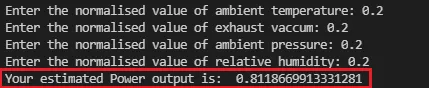
At 7000 iterations of linear regression.

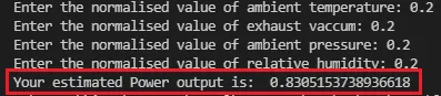
At 9000 iterations of linear regression.

Program without normalizing the data:

Dataset: https://drive.google.com/file/d/1a0QXjYk-ZXxE_a0zQu1urt7WbZGKcJSf/view?usp=sharing

# ERROR PROGRAMME
import numpy as np
import pandas as pd
import matplotlib.pyplot as plt
import seaborn as sns

df=pd.read_csv('data.csv')
# ambient_T 
x_1 = df.iloc[:, 0]
x1 = x_1/max(x_1)
# print(x1)

# exhaust_vaccum 
x_2 = df.iloc[:, 1]
x2 = x_2/max(x_2)
# ambient_P 
x_3 = df.iloc[:, 2]
x3 = x_3/max(x_3)
# relative_humidity 
x_4 = df.iloc[:, 3]
x4 = x_4/max(x_4)
# energy_output
y_ = df.iloc[:, 4]
y = y_/max(y_)
#print(y)

iter = 1000
m = np.zeros((4,1))
c = np.zeros((4,1))
learning_rate = 0.0001
n = len(df)

# to check if there are any null values in the dataset
print(df.isnull())

print('Size of data matrix: ', df.shape)
print(df.head())

"""plt.scatter(ambient_T, energy_output)
plt.show()"""

# data distribution of energy output
sns.displot(np.log10(df['PE']))
plt.show()



m_one = m[0]
m_two = m[1]
m_three = m[2]
m_four = m[3]

c_one = c[0]
c_two = c[1]
c_three = c[2]
c_four = c[3]







L = 0.0001  # Learning Rate
iter = 1000  # Number of iterations to perform gradient descent
n = len(x1) # Number of elements in X
print(n)
# def simple_linear_regression():

m_empty = []
c_empty = []

for i in range(50):

    y_pred_one = m_one*x1 + c_one
    # print(y_pred)
    y_pred_two = m_two*x2 + c_two
    y_pred_three = m_three*x3 + c_three
    y_pred_four = m_four*x4 + c_four

    D_m_one = -(2/n) * np.sum(1 * (y - y_pred_one))
    # print('dm = ', D_m)
    D_c_one = -(2/n) * np.sum(y - y_pred_one)
    # print(D_c)

    D_m_two = -(2/n) * np.sum(x2 * (y - y_pred_two))
    D_c_two = -(2/n) * np.sum(y - y_pred_two)

    D_m_three = -(2/n) * np.sum(x3 * (y - y_pred_three))
    D_c_three = -(2/n) * np.sum(y - y_pred_three)

    D_m_four = -(2/n) * np.sum(x4 * (y - y_pred_four))
    D_c_four = -(2/n) * np.sum(y - y_pred_four)

    m_one = m_one - L* D_m_one
    c_one = c_one - L* D_c_one

    m_two = m_two - L* D_m_two
    c_two = c_two - L* D_c_two

    m_three = m_three - L* D_m_three
    c_three = c_three - L* D_c_three

    m_four = m_four - L* D_m_four
    c_four = c_four - L* D_c_four

    h = D_m_one * x1 + D_m_two * x2 + D_m_three * x3 + D_m_four * x4
    print('h = ', h)


print(m_one, c_one)
print(m_two, c_two)
print(m_three, c_three)
print(m_four, c_four)

y_pred_one = m_one*x1 + c_one
y_pred_two = m_two*x2 + c_two
y_pred_three = m_three*x3 + c_three
y_pred_four = m_four*x4 + c_four

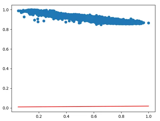
plt.scatter(x1, y)
plt.plot([min(x1), max(x1)], [min(y_pred_one), max(y_pred_one)], color='red')  # regression line
plt.show()

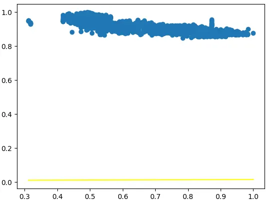
plt.scatter(x2, y)
plt.plot([min(x2), max(x2)], [min(y_pred_two), max(y_pred_two)], color='yellow')  # regression line
plt.show()

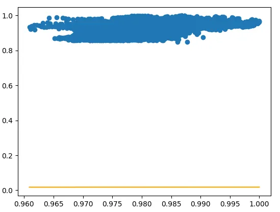
plt.scatter(x3, y)
plt.plot([min(x3), max(x3)], [min(y_pred_three), max(y_pred_three)], color='orange')  # regression line
plt.show()

plt.scatter(x4, y)
plt.plot([min(x4), max(x4)], [min(y_pred_four), max(y_pred_four)], color='green')  # regression line
plt.show()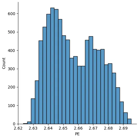

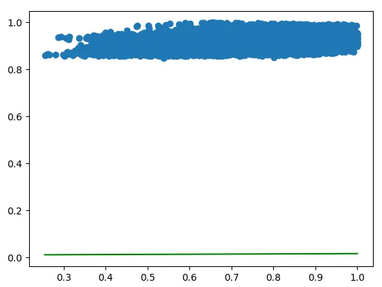
2. Difference between L1 & L2 Gradient descent method

Mean absolute error (MAE) = L1
In simple terms, mean absolute error is the sum of absolute/positive errors of all values. So, if there are 5 values in our data set, we find out the difference between the actual value and predicted values for all 5 values and take their positive value. So even if the difference between actual and predicted value is negative, we take positive value for calculation.

So we take the positive value of all errors, add them and find out their mean.

Mean absolute error illustration;

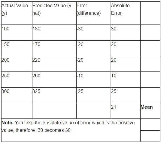
MAE is the sum of absolute differences between actual and predicted values. It doesn’t consider the direction, that is, positive or negative.
When we consider directions also, that is called Mean Bias Error (MBE), which is a sum of errors(difference).

Formula for mean absolute Error or MAE is represented by;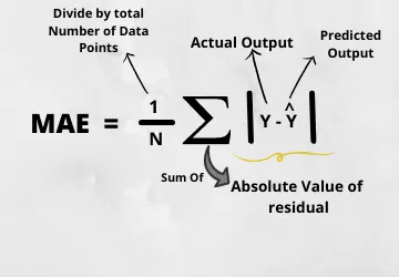

Mean Square Error (MSE) = L2
Mean square error is always positive and a value closer to 0 or a lower value is better.

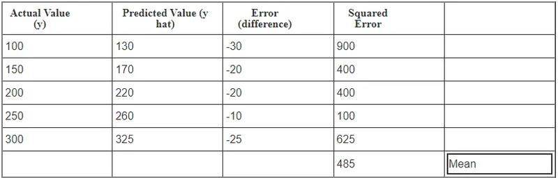
Formula for mean absolute Error or MSE is represented by;

So if we were to run a model with different parameters/independent variables, model with lower MSE will be deemed better.

3. What are the different loss functions for regression

Regression loss

• MSE
• MAE
• Huber loss
• Log cosh loss
• Quantile loss

1. Mean Square Error or L2 Loss:
Mean Square Error (MSE) is the most commonly used regression loss function. MSE is the sum of squared distances between our target variable and predicted values.

2. Mean Absolute Error, L1 Loss:
Mean Absolute Error (MAE) is another loss function used for regression models. MAE is the sum of absolute differences between our target and predicted variables. So it measures the average magnitude of errors in a set of predictions, without considering their directions. (If we consider directions also, that would be called Mean Bias Error (MBE), which is a sum of residuals/errors). The range is also 0 to ∞.

3. Huber Loss:
Huber loss is also called Smooth Mean Absolute Error. This loss function is less sensitive to outliers in data than the squared error loss. It’s also differentiable at 0. It’s basically absolute error, which becomes quadratic when error is small. How small that error has to be to make it quadratic depends on a hyperparameter, 𝛿 (delta), which can be tuned. Huber loss approaches MSE when 𝛿 ~ 0 and MAE when 𝛿 ~ ∞ (large numbers.)

4. Log-Cosh Loss
Log-cosh is another function used in regression tasks that’s smoother than L2. Log-cosh is the logarithm of the hyperbolic cosine of the prediction error.

5. Quantile Loss
In most of the real world prediction problems, we are often interested to know about the uncertainty in our predictions. Knowing about the range of predictions as opposed to only point estimates can significantly improve decision making processes for many business problems.

Quantile loss functions turn out to be useful when we are interested in predicting an interval instead of only point predictions. Prediction interval from least square regression is based on an assumption that residuals (y — y) have constant variance across values of independent variables. We can not trust linear regression models which violate this assumption. We can not also just throw away the idea of fitting linear regression model as baseline by saying that such situations would always be better modeled using non-linear functions or tree based models. This is where quantile loss and quantile regression come to rescue as regression based on quantile loss provides sensible prediction intervals even for residuals with non-constant variance or non-normal distribution.

4. What is the importance of learning rate

Learning rate is a parameter, denoted by α(alpha), is used to tune how accurately a model converges on a result (classification/prediction, etc.). This can be thought of as a ball thrown down a staircase. And a higher learning rate value is equivalent to the higher speed of the descending ball. This ball will leap skipping adjacent steps, and reaching the bottom quickly but not settling immediately because of the momentum it carries.

Learning rate is a scalar, a value which tells the machine how fast or how slow to arrive at some conclusion. The speed at which a model learns is important and it varies with different applications. A super fast learning algorithm can miss a few data points or correlations which can give better insights on the data. Missing this will eventually lead to wrong classifications.

And, to find the next step or the adjacent data point, the gradient descent algorithms multiply the gradient by learning rate (also called step size).

For example, if the gradient magnitude is 1.5 and the learning rate is 0.01, then the gradient descent algorithm will pick the next point 0.015 away from the previous point.

If a learning rate is too small, learning will take too long:

And if a learning rate is too large, the next point will perpetually bounce haphazardly across the bottom of the valley:

This momentum can be controlled with three common types of implementing the learning rate decay:

1. Step decay: Reduce the learning rate by some factor every few epochs. Typical values might be reducing the learning rate by a half every 5 epochs, or by 0.1 every 20 epochs.
2. Exponential decay has the mathematical form α=α_0e^(−kt), where α_0,k are hyperparameters and t is the iteration number.
3. 1/t decay has the mathematical form α=α0/(1+kt) where a0,k are hyperparameters and t is the iteration number.

5. How to evaluate linear regression

Linear regression is a regression model that uses a straight line to describe the relationship between variables. It finds the line of best fit through your data by searching for the value of the regression coefficient(s) that minimizes the total error of the model.

There are two main types of linear regression:

• Simple linear regression uses only one independent variable
• Multiple linear regression uses two or more independent variables

In this step-by-step guide, we will walk you through linear regression in R using two sample datasets.

There are three error metrics that are commonly used for evaluating and reporting the performance of a regression model; they are:

• Mean Squared Error (MSE).
• Root Mean Squared Error (RMSE).
• Mean Absolute Error (MAE)

There are many other metrics for regression, although these are the most commonly used. You can see the full list of regression metrics supported by the scikit-learn Python machine learning library here: https://scikit-learn.org/stable/modules/classes.html#regression-metrics

Step#1 Importing the required libraries

Step#2 Loading the dataset

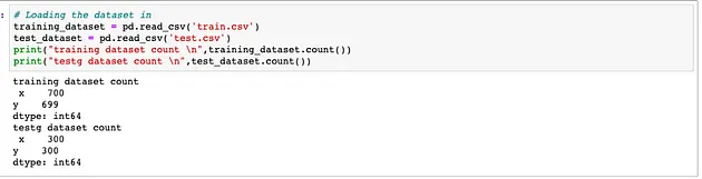
Step#3 Let’s check for any missing or NA values in the training and testing data set

We can see that there is a missing value for Y.

Let’s check for any missing or NA values in the training and testing data set

There is no missing value in the test data.

Step#4 Let’s drop the record with missing value in the training dataset. As it is only one record, removing it will not be much of concern.

Now the x and y values are equal in the training data set.

Step#5 Let’s check for useful descriptive statistical values

Applying pandas “describe()” function

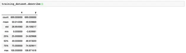
We have total records count, mean, median, standard deviation, and quartiles for our training data.

Step#6 Let’s define our dependent and independent variable for training and testing data

Step#7 Let’s explore the relationship between the dependent variable and the independent variable.

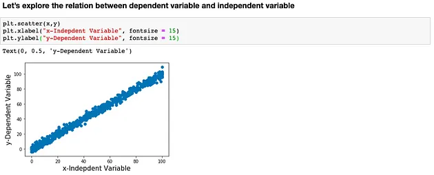
Above graphical depictions is clearly showing a very strong relationship between the dependent and independent variable

Step#8 Let’s add a constant, to add a constant we will create a new variable.

As we know linear regression is typically as follows:

y = a + bx,

Since we already have “y” and “x”, here we are trying to create “a” by adding a constant to our dataset. It is computationally important. We will be leveraging the “add_constant()” function of statsmodel library.

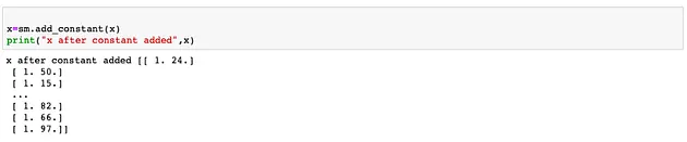
Above image shows the “1” added as a constant

Step#9 Let’s define the model and fit it.

We will be defining our first model and for this model, we will be leveraging “statsmodels” library.

Defining a variable named “Model1” to store the result

Step#10 Let’s look at different parameters of the model summary and interpret it:

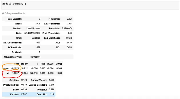
From “Model1” summary we got “const” and “x1”, which are helping to create our final regression equation

“y=-0.1073+1.0007x”

Step#11 Let’s define our final regression equation using model output parameters

Step#12: Now let’s visualise the regression equation fitment on the data

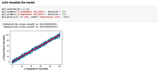
Step#13: Now let’s check how our model is doing on the testing data, which we kept aside for testing our model performance

Here, we have defined a variable named “df” to store the actual and predicted values in a data frame.

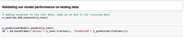
Step#14: Final step to visualise the Model1 performance against various well-established evaluation metrics

For regression problems following three metrics are used:

1.Mean Absolute Error (MAE) is the mean of the absolute value of the errors. It is calculated as:

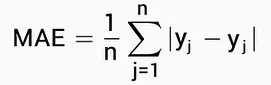
2. Mean Absolute Error

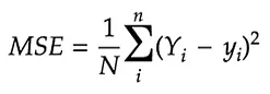
Best value for this is 0.0

3. Mean Squared Error (MSE) is the mean of the squared errors and is calculated as:

Root Mean Squared Error (RMSE) is the square root of the mean of the squared errors.

Best value for this is 0.0

We got following :

Mean Absolute Error: 2.4157718500412586

Mean Squared Error: 9.432922192039317

Root Mean Squared Error: 3.0713062680298293

6. What is the difference between multiple and adjusted coefficient of determination

Coefficient of determination:

In statistics, the coefficient of determination, denoted `R^2 or r^2` and pronounced "R squared", is the proportion of the variation in the dependent variable that is predictable from the independent variable(s).

It is a statistic used in the context of statistical models whose main purpose is either the prediction of future outcomes or the testing of hypotheses, on the basis of other related information. It provides a measure of how well observed outcomes are replicated by the model, based on the proportion of total variation of outcomes explained by the model.

Multiple R squared is simply a measure of Rsquared for models that have multiple predictor variables. Therefore it measures the amount of variation in the response variable that can be explained by the predictor variables. The fundamental point is that when you add predictors to your model, the multiple Rsquared will always increase, as a predictor will always explain some portion of the variance.

Adjusted Rsquared controls against this increase, and adds penalties for the number of predictors in the model. Therefore it shows a balance between the most parsimonious model, and the best fitting model. Generally, if you have a large difference between your multiple and your adjusted Rsquared that indicates you may have overfit your model.

References:

Linear regression: Single variable

https://www.youtube.com/watch?v=8jazNUpO3lQ

Linear regression: Multi variable

https://www.youtube.com/watch?v=J_LnPL3Qg70

Other references:

https://www.geeksforgeeks.org/bin-size-in-matplotlib-histogram/

https://vitalflux.com/gradient-descent-explained-simply-with-examples/#Introduction_to_Gradient_Descent_Algorithm

https://towardsdatascience.com/gradient-descent-algorithm-a-deep-dive-cf04e8115f21

https://machinelearningmastery.com/gradient-descent-for-machine-learning/

https://www.ibm.com/cloud/learn/gradient-descent

https://akhilendra.com/evaluation-metrics-regression-mae-mse-rmse-rmsle/

https://inblog.in/Top-10-activation-and-loss-function-which-you-should-know-about-it-wM27n7JXRg

https://analyticsindiamag.com/why-learning-rate-is-crucial-in-deep-learning/

https://www.ritchieng.com/machine-learning-evaluate-linear-regression-model/

https://medium.com/@mygreatlearning/step-by-step-regression-analysis-f7e3e3ebf296

https://stats.stackexchange.com/questions/241283/what-is-the-main-difference-between-multiple-r-squared-and-adjusted-r-squared