Week 11 - Simulation of Flow through a pipe in OpenFoam
Expected Results :
Code in Matlab to automate the generation of blockMeshDict file.
- Validate Hydro-dynamic length with the numerical result .
- Validate the fully developed flow velocity profile with its analytical profile .
- Validate maximum velocity and pressured drop for fully developed flow .
- Post-process Shear stress and validate wall shear stress for fully developed flow.
Assumptions :
1 . Diameter of the pipe : 0.02m .
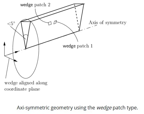
2 . Wedge angle : `theta`: 3 degrees .
3 . Working fluid medium : Water .
4 . Temprature of water : 20 degrees .
Density(at 20deg C) : `rho`=998.23 kg/m^3
Dynamic viscosity(at 20deg C) : `mu`=0.001002 kg/m.s
Kinematic viscosity(at 20deg C) : `nu`=0.000001002 m^2/s
5 . Axi-symmetric flow & laminar and flows through a constant cross-section pipe at an inlet Reynold's number of 2100 .
Formulas for simulating Hagen-Poiseuille flow in a pipe :
- Pressure change : `DeltaP=(32muoverlineu(L-L_e))/D^2`
- Entry length :`L_e=0.06*Re*D`
- Length of pipe :`L =0.5+L_e`
- Kinematic pressure : `(DeltaP)/rho_(at T^oC)`
- Average fluid velocity : `V_(avg)=overlineV=(Re*mu)/(rho*D)`
- Shear stress : `tau=-mu(du)/(dy)`
Pipe geometry :
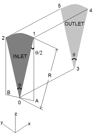
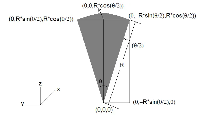
Vertices :
Y distance :
Cosider angle `theta/2`
`cos(theta/2)=(1A)/R`
`R*cos(theta/2)=1A`= Vertical component
X distance :
Cosider angle `theta/2`
`sin(theta/2)=(0A)/R`
`R*sin(theta/2)=0A` = Horizontal component
Developing flow and fully developed flow :
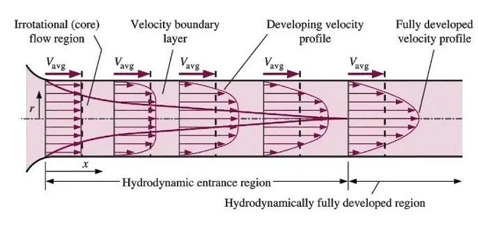
Flow in a conduit is classified as being developing flow or fully developed flow. For example, considering a laminar fluid entering a pipe, as the fluid moves down the pipe, the velocity distribution changes in the stream wise direction as viscous effects cause the plug type profile to gradually change into a parabolic profile. This region of changing velocity profile is called developing flow. After the parabolic distribution is achieved, the flow profile remains unchanged in the stream wise direction, and the flow is called fully developed flow.The distance required for a flow to develop is called the entrance length(Le), and depends on the shear stresses that act on the pipe wall .
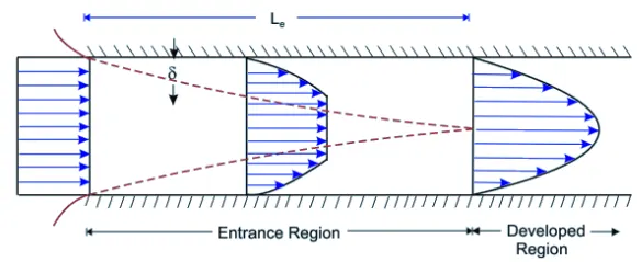
Near the pipe entrance, the radial velocity gradient (change in velocity with distance from the wall) is high, so the shear stress is large. As the velocity profile progresses to a parabolic shape, the velocity gradient and the wall shear stress decrease until a constant value is achieved. The entry length is defined as the distance at which the shear stress reaches to within 2% of the fully developed value.Correlations for entry length are:
Laminar Flow : `L_e/D=0.05Re`
Turbulent Flow : `L_e/D=4.4 (Re)^(1/6)`
These values are only valid for a flow entering a circular pipe from quiet conditions. If some other elements like valves, elbows or pumps are present, different entrance lengths will occur.
Pressure loss during laminar flow in a pipeline :
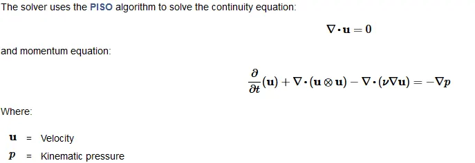
For laminar flow it is possible to calculate a theoretical value for a given velocity, fluid and pipe dimension. The pressure loss in a pipe with laminar flow is given by the Hagen-Poiseuille equation :
`DeltaP=(32muoverlineu(L-L_e))/D^2`
Where,
`DeltaP`=Pressure difference .
`mu`=Viscosity of fluid
`overlineu`=Average velocity of fluid
`L`=Length of pipe
`L_e`=Entrance length
D=Diameter of the pipe
Reynolds number :
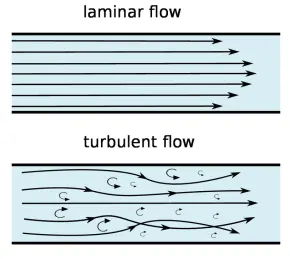
For pipe flow applications, it’s often important to be able to determine whether a given flow condition is laminar flow or turbulent flow. Different equations or methods of analysis often apply to laminar flow and turbulent flow conditions.
The typical criterion for whether pipe flow is laminar or turbulent is the value of the Reynolds Number. The Reynolds number for pipe flow is defined as
`Re = (DVrho)/mu` = `uL/nu`
where D is the pipe diameter,
V is the average flow velocity in the pipe,
`rho` is the density of the flowing fluid
and
`mu` is the dynamic viscosity of the flowing fluid.
`nu`is the kinematic viscosity =`rho/mu=1/nu`
Re is a dimensionless number.
Any consistent set of units can be used for D, V, `rho` and , and will result in Reynolds number being dimensionless. The generally accepted criteria for laminar flow and turbulent flow in terms of Re are as follows:
For Re < 2100, it is laminar flow.
For Re > 4000, it is turbulent flow.
For 2100 < Re < 4000, the flow is in the transition region.
For flow in the transition region, the flow may be either laminar or turbulent, depending upon the nature of the entrance to the pipe and the pipe wall roughness.
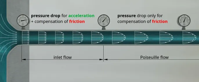
Why the equation of Hagen-Poiseuille does not apply in the inlet of a pipe .
A pressure drop between the beginning and the end of a pipe is the drive for a flow. However, the pressure gradient that forms over the length of the pipe has two tasks, so to speak. The pressure drop must not only compensate the frictional force during the flow of the fluid, but must accelerate the fluid to achieve the characteristic flow profile in the first place.
Therefore, the total pressure drop can be divided into a part which is used to accelerate the fluid and a part which is used to compensate for friction. In the above equations, the pressure gradient dp/dx only refers to that part of the total pressure gradient which is necessary to overcome the friction.
To determine this pressure gradient, one must not simply take the pressure difference between the beginning and end of the pipe and then divide it by the length of the pipe. This is why the above equations always referred to a pipe section where it was implicitly assumed that the parabolic flow profile had already been fully established.
The equation of Hagen-Poiseuille does not apply in the inlet of a pipe (inlet flow), within which the pressure gradient must accelerate the fluid to the typical parabolic profile in addition to overcoming friction .
Under certain circumstances, it may nevertheless be justified to describe flow by simply determining the pressure gradient in the above equations from the quotient of pressure drop and pipe length. Namely, whenever the work of acceleration is negligible compared to the friction work. This will always be the case if the pipe is relatively long compared to its diameter, or if the flow velocities are relatively low. In such cases, the frictional work usually clearly outweighs the relatively low work of acceleration due to the long pipe length.
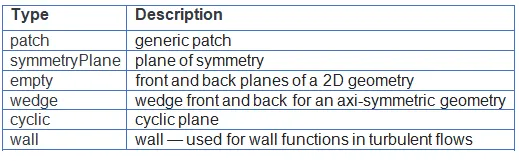
Boundary types :
patch :
The basic patch type for a patch condition that contains no geometric or topological information about the mesh (with the exception of wall), e.g. an inlet or an outlet.
symmetryPlane :
For a symmetry plane.
empty :
While OpenFOAM always generates geometries in 3 dimensions, it can be instructed to solve in 2 (or 1) dimensions by specifying a special empty condition on each patch whose plane is normal to the 3rd (and 2nd) dimension for which no solution is required.
wedge :
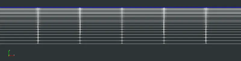
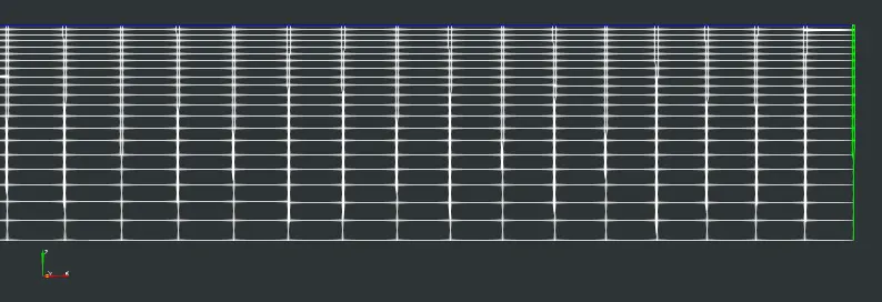
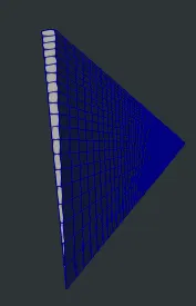
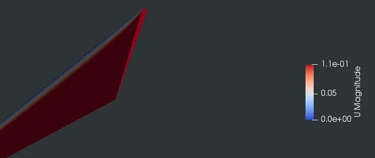
For 2 dimensional axi-symmetric cases, e.g. a cylinder, the geometry is specified as a wedge of small angle (e.g. 5 degrees) and 1 cell thick running along the plane of symmetry, straddling one of the coordinate planes. The axi-symmetric wedge planes must be specified as separate patches of wedge type. The details of generating wedge-shaped geometries using blockMesh .
Remember to specify the wedges seperately under 'boundary' in blockMesDict file .
Below is the link to the copy of the error dialogue from the ubuntu terminal that appeared because of putting the 2 wedges together.
https://drive.google.com/file/d/1ERrvkwyu9LZgv2ymP65O4NKCo67KGjgN/view?usp=sharing
cyclic :
Enables two patches to be treated as if they are physically connected; used for repeated geometries, e.g. heat exchanger tube bundles. One cyclic patch is linked to another through a neighbourPatch keyword in the boundary file. Each pair of connecting faces must have similar area to within a tolerance given by the matchTolerance keyword in the boundary file. Faces do not need to be of the same orientation.
wall :
There are instances where a patch that coincides with a wall needs to be identifiable as such, particularly where specialist modelling is applied at wall boundaries. A good example is wall turbulence modelling where a wall must be specified with a wall patch type, so that the distance from the wall of the cell centres next to the wall are stored as part of the patch.
Here we will be using wall boundary to demonstrate noslip condition at the pipe wall.
Boundary and initial conditions :When solving circulating internal flow, the most common boundary con-ditions are to fix an inlet velocity and an outlet pressure (or viceversa).
Creating blocks with fewer than 8 vertices :
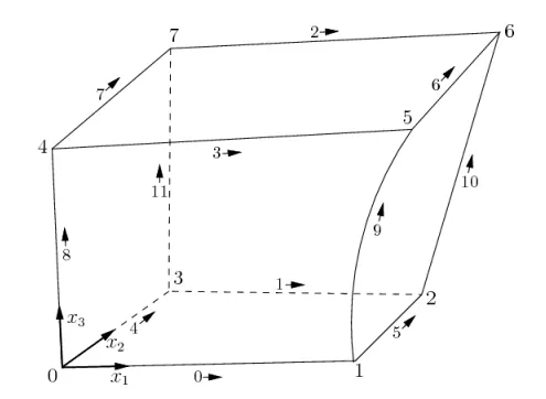
It is possible to collapse one or more pair(s) of vertices onto each other in order to create a block with fewer than 8 vertices. The most common example of collapsing vertices is when creating a 6-sided wedge shaped block for 2-dimensional axi-symmetric cases that use the wedge patch type. The process is best illustrated by using a simplified version of our example block shown in Figure below. Let us say we wished to create a wedge shaped block by collapsing vertex 7 onto 4 and 6 onto 5. This is simply done by exchanging the vertex number 7 by 4 and 6 by 5 respectively so that the block numbering would become : hex (0 1 2 3 4 5 5 4) .
The same applies to the patches with the main consideration that the block face containing the collapsed vertices, previously (4 5 6 7) now becomes (4 5 5 4). This is a block face of zero area which creates a patch with no faces in the polyMesh, as the user can see in a boundary file for such a case. The patch should be specified as empty in the blockMeshDict and the boundary condition for any fields should consequently be empty also.
The edges
Each edge joining 2 vertex points is assumed to be straight by default. However any edge may be specified to be curved by entries in a list named edges. The list is optional; if the geometry contains no curved edges, it may be omitted.
edges
(
arc 1 5 (1.1 0.0 0.5)
);
Simulation type :
- Steady-state simulation computes the fully developed solution that does not change in time.
- When steady-state used the mean values are computed.
- The steady-state simulation is the way faster than transient.
- Transient simulation computes the instantaneous values in each time for each quantity.
- Transient simulation has much higher requirements comparing to steady-state. The CPU time, disk storage, evaluating results.
- The results of transient simulation may be more comprehensive.
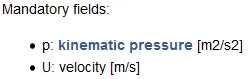
Solver : Solver used is icoFoam
Main code :
Refer to the below link for more information on file parsing on MATLAB :
https://www.mathworks.com/help/matlab/ref/textscan.html#btghhyz-1-formatSpec
clear all
close all
clc

Re=2100;
% Conidering standard room temprature of water as 20 degree celcius
rho=998.23;  %density(kg/m^3)at 20deg C
mu=0.001002;   %dynamic viscosity(kg/m.s)at 20deg C
v=0.000001002;  %kinematic viscosity(m^2/s)at 20deg C
prompt = 'Diameter of the pipe?';
D = input(prompt)
Le=0.06*Re*D
% total length of pipe
L=0.5+Le;
% angle of wedge
prompt = 'What is the wedge angle? ';
theta = input(prompt)
if theta>5
    theta=fprintf('Choose an angle lesser than 5 degrees');
end

a=(D/2)*sind(theta/2);
b=(D/2)*cosd(theta/2);

v0=[0,0,0];
v1=[0,-a,b];
v2=[0,a,b];
v3=[L,0,0];
v4=[L,-a,b];
v5=[L,a,b];

f1=fopen('blockMeshDict.txt','w')

fprintf(f1,'%s \n','/*--------------------------------*- C++ -*----------------------------------*\');
fprintf(f1,'%s \n','  =========                 |');
fprintf(f1,'%s \n','  \\      /  F ield         | OpenFOAM: The Open Source CFD Toolbox');
fprintf(f1,'%s \n','   \\    /   O peration     | Website:  https://openfoam.org');
fprintf(f1,'%s \n','    \\  /    A nd           | Version:  8');
fprintf(f1,'%s \n','     \\/     M anipulation  |');
fprintf(f1,'%s \n','\*---------------------------------------------------------------------------*/');
fprintf(f1,'%s \n','FoamFile');
fprintf(f1,'%s \n','{');
fprintf(f1,'%s \n','    version     2.0;');
fprintf(f1,'%s \n','    format      ascii;');
fprintf(f1,'%s \n','    class       dictionary;');
fprintf(f1,'%s \n','    object      blockMeshDict;');
fprintf(f1,'%s \n','}');
fprintf(f1,'%s \n','// * * * * * * * * * * * * * * * * * * * * * * * * * * * * * * * * * * * * * //');

% for one line space
fprintf(f1,'\n');
fprintf(f1,'%s \n','convertToMeters 1;');

fprintf(f1,'\n');
fprintf(f1,'%s \n','vertices');
fprintf(f1,'%s \n','(');
fprintf(f1,'(%f %f %f)\n',v0(1),v0(2),v0(3));
fprintf(f1,'(%f %f %f)\n',v1(1),v1(2),v1(3));
fprintf(f1,'(%f %f %f)\n',v2(1),v2(2),v2(3));
fprintf(f1,'(%f %f %f)\n',v3(1),v3(2),v3(3));
fprintf(f1,'(%f %f %f)\n',v4(1),v4(2),v4(3));
fprintf(f1,'(%f %f %f)\n',v5(1),v5(2),v5(3));
fprintf(f1,');');
fprintf(f1,'\n');

fprintf(f1,'\nblocks \n');
fprintf(f1,'%s \n','(');
fprintf(f1,'%s \n','hex (0 3 3 0 1 4 5 2) (400 1 20) simpleGrading ');
fprintf(f1,'%s \n','(');
fprintf(f1,'%s \n','(');
fprintf(f1,'%s \n','(20 30 4)');
fprintf(f1,'%s \n','(60 40 1)');
fprintf(f1,'%s \n','(20 30 0.25)');
fprintf(f1,'%s \n',')');
fprintf(f1,'%s \n','1');
fprintf(f1,'%s \n','0.25');
fprintf(f1,'%s \n',')');
fprintf(f1,');');
fprintf(f1,'\n');

fprintf(f1,'\nedges \n');
fprintf(f1,'%s \n','(');
% '%d' is used to represent integers
fprintf(f1,'arc %d %d (%d %d %d)\n',1,2,v2(1),v2(2),v2(3));
fprintf(f1,'arc %d %d (%d %d %d)\n',4,5,v5(1),v5(2),v5(3));
fprintf(f1,');');
fprintf(f1,'\n');

fprintf(f1,'\nboundary \n');
fprintf(f1,'%s \n','(');
% inlet
fprintf(f1,'inlet');
fprintf(f1,'\n');
fprintf(f1,'%s \n','{');
fprintf(f1,'%s','type patch;');
fprintf(f1,'\nfaces');
fprintf(f1,'\n');
fprintf(f1,'%s \n','(');
fprintf(f1,'(0 1 2 0)\n');
fprintf(f1,');');
fprintf(f1,'\n');
fprintf(f1,'}');
fprintf(f1,'\n');
% outlet
fprintf(f1,'outlet');
fprintf(f1,'\n');
fprintf(f1,'%s \n','{');
fprintf(f1,'%s','type patch;');
fprintf(f1,'\nfaces');
fprintf(f1,'\n');
fprintf(f1,'%s \n','(');
fprintf(f1,'(3 5 4 3)\n');
fprintf(f1,');');
fprintf(f1,'\n');
fprintf(f1,'}');
fprintf(f1,'\n');
% front
fprintf(f1,'front');
fprintf(f1,'\n');
fprintf(f1,'%s \n','{');
fprintf(f1,'%s','type wedge;');
fprintf(f1,'\nfaces');
fprintf(f1,'\n');
fprintf(f1,'%s \n','(');
fprintf(f1,'(0 3 4 1)\n');
fprintf(f1,');');
fprintf(f1,'\n');
fprintf(f1,'}');
fprintf(f1,'\n');
% back
fprintf(f1,'back');
fprintf(f1,'\n');
fprintf(f1,'%s \n','{');
fprintf(f1,'%s','type wedge;');
fprintf(f1,'\nfaces');
fprintf(f1,'\n');
fprintf(f1,'%s \n','(');
fprintf(f1,'(0 2 5 3)\n');
fprintf(f1,');');
fprintf(f1,'\n');
fprintf(f1,'}');
fprintf(f1,'\n');
% axis
fprintf(f1,'axis');
fprintf(f1,'\n');
fprintf(f1,'%s \n','{');
fprintf(f1,'%s','type empty;');
fprintf(f1,'\nfaces');
fprintf(f1,'\n');
fprintf(f1,'%s \n','(');
fprintf(f1,'(0 3 3 0)\n');
fprintf(f1,');');
fprintf(f1,'\n');
fprintf(f1,'}');
fprintf(f1,'\n');
% top
fprintf(f1,'top');
fprintf(f1,'\n');
fprintf(f1,'%s \n','{');
fprintf(f1,'%s','type wall;');
fprintf(f1,'\nfaces');
fprintf(f1,'\n');
fprintf(f1,'%s \n','(');
fprintf(f1,'(1 4 5 2)\n');
fprintf(f1,');');
fprintf(f1,'\n');
fprintf(f1,'}');
fprintf(f1,'\n');
fprintf(f1,'%s \n',');');

fprintf(f1,'\n');
fprintf(f1,'mergePatchPairs');
fprintf(f1,'\n(');
fprintf(f1,'\n);');
fprintf(f1,'\n// ************************************************************************* //');
blockMeshDict file :
/*--------------------------------*- C++ -*----------------------------------*\
  =========                 |
  \\      /  F ield         | OpenFOAM: The Open Source CFD Toolbox
   \\    /   O peration     | Website:  https://openfoam.org
    \\  /    A nd           | Version:  8
     \\/     M anipulation  |
\*---------------------------------------------------------------------------*/
FoamFile
{
    version     2.0;
    format      ascii;
    class       dictionary;
    object      blockMeshDict;
}
// * * * * * * * * * * * * * * * * * * * * * * * * * * * * * * * * * * * * * //

convertToMeters 1;

vertices
(
(0.000000 0.000000 0.000000)
(0.000000 -0.000262 0.009997)
(0.000000 0.000262 0.009997)
(3.020000 0.000000 0.000000)
(3.020000 -0.000262 0.009997)
(3.020000 0.000262 0.009997)
);

blocks
(
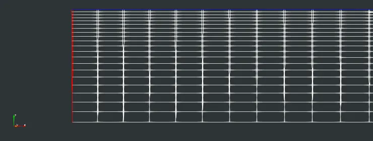
hex (0 3 3 0 1 4 5 2) (400 1 20) simpleGrading
(
(
(20 30 4)
(60 40 1)
(20 30 0.25)
)
1
0.25
)
);

edges
(
arc 1 2 (0 2.617695e-04 9.996573e-03)
arc 4 5 (3.020000e+00 2.617695e-04 9.996573e-03)
);

boundary
(
inlet
{
type patch;
faces
(
(0 1 2 0)
);
}
outlet
{
type patch;
faces
(
(3 5 4 3)
);
}
front
{
type wedge;
faces
(
(0 3 4 1)
);
}
back
{
type wedge;
faces
(
(0 2 5 3)
);
}
axis
{
type empty;
faces
(
(0 3 3 0)
);
}
top
{
type wall;
faces
(
(1 4 5 2)
);
}
);

mergePatchPairs
(
);
// ************************************************************************* //
Pressure file :
/*--------------------------------*- C++ -*----------------------------------*\
  =========                 |
  \\      /  F ield         | OpenFOAM: The Open Source CFD Toolbox
   \\    /   O peration     | Website:  https://openfoam.org
    \\  /    A nd           | Version:  8
     \\/     M anipulation  |
\*---------------------------------------------------------------------------*/
FoamFile
{
    version     2.0;
    format      ascii;
    class       volScalarField;
    object      p;
}
// * * * * * * * * * * * * * * * * * * * * * * * * * * * * * * * * * * * * * //

dimensions      [0 2 -2 0 0 0 0];

internalField   uniform 0;

boundaryField
{
    inlet
    {
        type            zeroGradient;
    }

    outlet
    {
        type            fixedValue;
	value    	 uniform 0;

    }

    front
    {
        type            wedge;
    }
    back
    {
        type            wedge;
    }
    axis
    {
        type            empty;
    }
    top
    {
        type            zeroGradient;
    }
}

// ************************************************************************* //
Velocity file :
/*--------------------------------*- C++ -*----------------------------------*\
  =========                 |
  \\      /  F ield         | OpenFOAM: The Open Source CFD Toolbox
   \\    /   O peration     | Website:  https://openfoam.org
    \\  /    A nd           | Version:  8
     \\/     M anipulation  |
\*---------------------------------------------------------------------------*/
FoamFile
{
    version     2.0;
    format      ascii;
    class       volVectorField;
    object      U;
}
// * * * * * * * * * * * * * * * * * * * * * * * * * * * * * * * * * * * * * //

dimensions      [0 1 -1 0 0 0 0];

internalField   uniform (0 0 0);

boundaryField
{
    inlet
    {
        type            fixedValue;
        value           uniform (0.1054 0 0);
    }

    outlet
    {
      	type 		 zeroGradient;
    }

    front
    {
        type            wedge;
    }
    back
    {
        type            wedge;
    }
    axis
    {
        type            empty;
    }
    top
    {
        type            noSlip;
    }
}

// ************************************************************************* //
controlDict file :
Calculation to determine endTime :
This is very important for endTime to be suffeciently large because it allows the fluid to pass through the entire section of the pipe
Velocity = Distance / Time
Time = Distance / Velocity
Distance from inlet to outlet of the pipe section : 3.02m
We know that velocity calculated is 0.1054 m/s from calculation
Time = 3.02/0.1054
= 28.64 s
So for the flow to completely pass through the pipe we need to give double or triple the amount of time given for the simulation to take place .
Hence 58s is used as endTime for the flow to take place from end to end length of the pipe .
/*--------------------------------*- C++ -*----------------------------------*\
  =========                 |
  \\      /  F ield         | OpenFOAM: The Open Source CFD Toolbox
   \\    /   O peration     | Website:  https://openfoam.org
    \\  /    A nd           | Version:  8
     \\/     M anipulation  |
\*---------------------------------------------------------------------------*/
FoamFile
{
    version     2.0;
    format      ascii;
    class       dictionary;
    location    "system";
    object      controlDict;
}
// * * * * * * * * * * * * * * * * * * * * * * * * * * * * * * * * * * * * * //

application     icoFoam;

startFrom       startTime;

startTime       0;

stopAt          endTime;

endTime         58;

deltaT          0.01;

writeControl    timeStep;

writeInterval   20;

purgeWrite      0;

writeFormat     ascii;

writePrecision  6;

writeCompression off;

timeFormat      general;

timePrecision   6;

runTimeModifiable true;


// ************************************************************************* //
transportProperties :
/*--------------------------------*- C++ -*----------------------------------*\
  =========                 |
  \\      /  F ield         | OpenFOAM: The Open Source CFD Toolbox
   \\    /   O peration     | Website:  https://openfoam.org
    \\  /    A nd           | Version:  8
     \\/     M anipulation  |
\*---------------------------------------------------------------------------*/
FoamFile
{
    version     2.0;
    format      ascii;
    class       dictionary;
    location    "constant";
    object      transportProperties;
}
// * * * * * * * * * * * * * * * * * * * * * * * * * * * * * * * * * * * * * //

nu              [0 2 -1 0 0 0 0] 1.002E-06;


// ************************************************************************* //
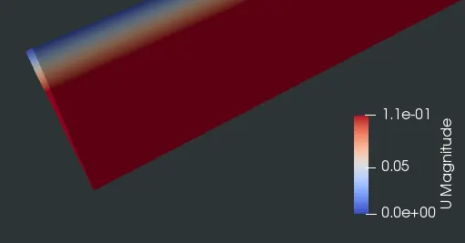
Velocity in radial direction :
At
x1 = 0 m ,x2 = 0 m
y1 = 0 ,y2 = 0
z1 = 0,z2 = 0.01
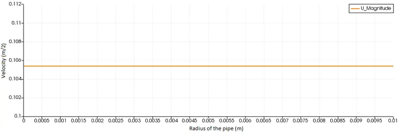
At
x1 = 0.1 m ,x2 = 0.1 m
y1 = 0 ,y2 = 0
z1 = 0,z2 = 0.01
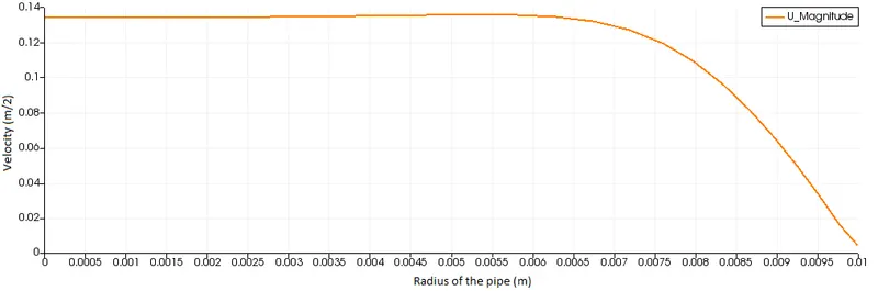
At
x1 = 0.25 m ,x2 = 0.25 m
y1 = 0 ,y2 = 0
z1 = 0,z2 = 0.01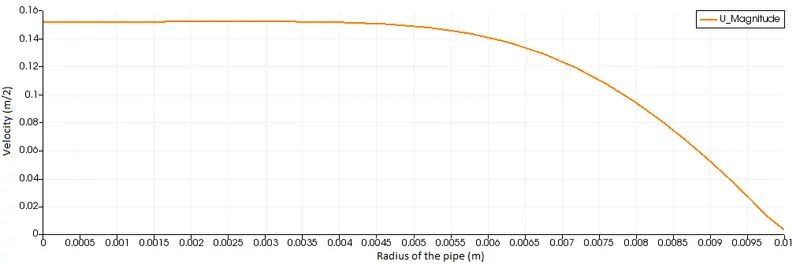
At
x1 = 0.5 m ,x2 = 0.5 m
y1 = 0 ,y2 = 0
z1 = 0,z2 = 0.01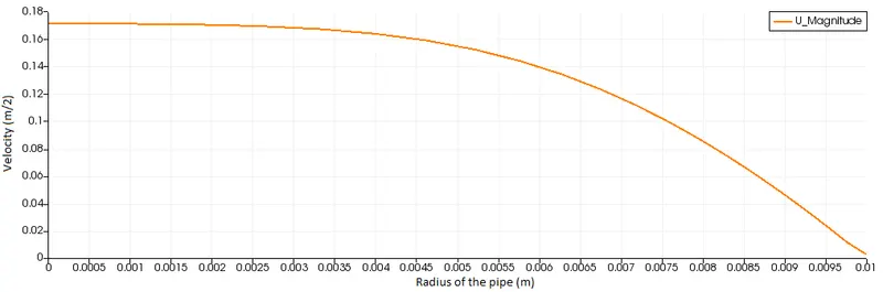
At
x1 = 1 m ,x2 = 1 m
y1 = 0 ,y2 = 0
z1 = 0,z2 = 0.01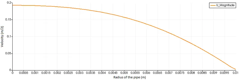
At
x1 = 1.5 m ,x2 = 1.5 m
y1 = 0 ,y2 = 0
z1 = 0,z2 = 0.01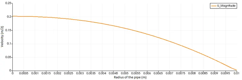
At
x1 = 2 m ,x2 = 2 m
y1 = 0 ,y2 = 0
z1 = 0,z2 = 0.01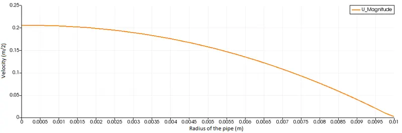
At
x1 = 2.5 m ,x2 = 2.5 m
y1 = 0 ,y2 = 0
z1 = 0,z2 = 0.01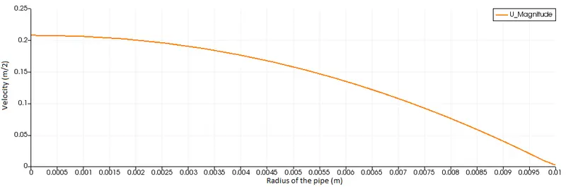
At
x1 = 3 m ,x2 = 3 m
y1 = 0 ,y2 = 0
z1 = 0,z2 = 0.01
Fully developed flow
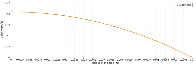
Analytical velocity value :
`Velocity_(avg) =(Re*mu)/(rho*D)`
`Velocity_(avg) = (2100*1.002*10^(-3))/(998.23*0.02)`
`Velocity_(avg) =0.1054m/s`
`V_max=2*Velocity_(avg)`
`V_max=0.2108m/s`
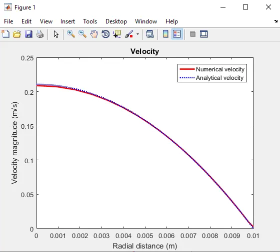
When we compare the analytical value of velocity with numerically obtained velocity there is not much difference .
Pressure in flow direction at fully developed region (from 2.52m to 3.02 m)
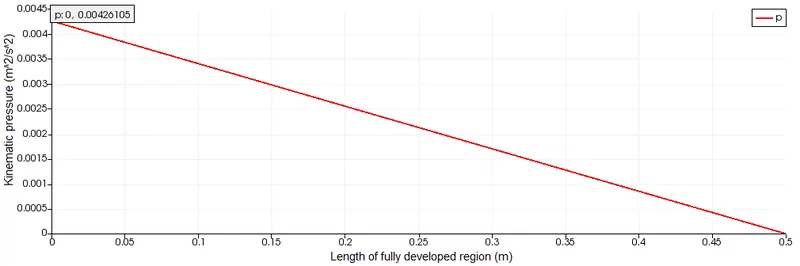
`DeltaP=(32muoverlineu(L-L_e))/D^2`
`Delta P=(32*0.001002*0.1054*0.5)/(0.02)^2`
`DeltaP=4.2243 Pa`
Kinematic pressure = `(DeltaP)/rho_(20C)=(4.2243/998.23) = 0.00423 m^2/s^2`
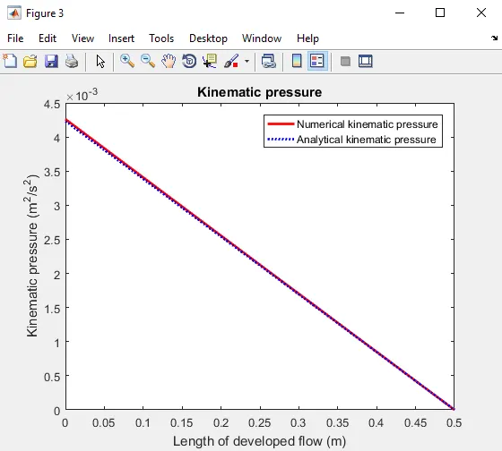
It's safe to safe to say that the analytical and numerical values for kinematic pressure when compared give us satisfactory results .
Shear stress in radial direction :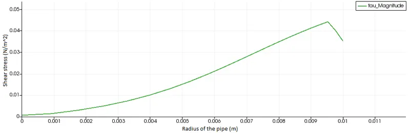
Post processing help for plotting shear stress on openfoam
https://skill-lync.freshdesk.com/support/solutions/articles/43000570187-how-to-create-shear-stress-plot-inside-paraview-
The Newton's constitutive law, for any general geometry (including the flat plate above mentioned), states that shear tensor (a second-order tensor) is proportional to the flow velocity gradient
and the constant of proportionality is named dynamic viscosity.(the velocity is a vector, so its gradient is a second-order tensor):
`tau = -mu*(du)/(dy)`
where ,`tau`=Shear stress `(N/m^2)`
`mu`=Dynamic viscosity `((kg)/(m.s))`
`(du)/(dy)`=Change in flow velocity per change in distance above the boundary(here ,change in radius) .
Negative sign denotes the direction of the shear stress .
Matlab code to compare analytical and numerical values (at fully developed region):
clear all
close all
clc

% importing data generated from openfoam
% velocity
A=importdata('v_fully_developed.txt');
x1=A(:,1);
y1=A(:,2);
% shear stress
B=importdata('tau_final.txt');
x2=B(:,1);
y2=B(:,2);
% pressure
C=importdata('pressure.txt');
x3=C(:,1);
y3=C(:,2);

% Generating analytical data from formula

mu=1.002*10^(-3);
v_mean=0.1054;
Lt=3.02;
Le=2.52;
L=Lt-Le;
p_x=linspace(0,L,1001);
D=0.02;
rho=998.23;

for i=1:length(p_x)
p(i)=(32*mu*v_mean*p_x(i))/(0.02)^2;
p_kinematic(i)=p(i)/rho;
end
p_kinematic_y = fliplr(p_kinematic);


dr=linspace(0,0.01,1001);
R=D/2;
% velocity
vmax=0.2107;
u_mag=vmax*(1-(dr.^2./R^2));
% shear stress
for i=2:length(dr)
du(i)=u_mag(i-1)-u_mag(i);
ddr(i)=dr(i-1)-dr(i);
tau(i)=-0.001002*du(i-1)/ddr(i-1);
end

figure(1)
plot(x1,y1,'r','LineWidth',2)
xlabel('Radial distance (m)')
ylabel('Velocity magnitude (m/s)')
hold on
plot(dr,u_mag,':b','LineWidth',2)
legend('Numerical velocity','Analytical velocity')
title('Velocity')

figure(2)
plot(x2,y2,'r','LineWidth',2)
xlabel('Radial distance (m)')
ylabel('Shear stress magnitude (N/m^2)')
hold on
plot(dr,tau,':b','LineWidth',2)
legend('Numerical shear stress','Analytical shear stress')
title('Shear stress')

figure(3)
plot(x3,y3,'r','LineWidth',2)
xlabel('Length of developed flow (m)')
ylabel('Kinematic pressure (m^2/s^2)')
hold on
plot(p_x,p_kinematic_y,':b','LineWidth',2)
legend('Numerical kinematic pressure','Analytical kinematic pressure')
title('Kinematic pressure')
Velocity file with imported data from openfoam :
https://drive.google.com/file/d/1EUUx5AHG-bNyzq1kTkwj6EqtTvlxF27B/view?usp=sharing
Shear stress with imported data from openfoam :
https://drive.google.com/file/d/1fWZkp9U_DHAN1mIxGYwEYTxaLM1Uzbu8/view?usp=sharing
Pressure file with imported data from openfoam :
https://drive.google.com/file/d/1NS1VHHr_4mP8HbaN10C3p2c_ZyvLb1OP/view?usp=sharing
Conclusion :
- We can clearly observe how the velocity profile stabilises after reaching entrance region .
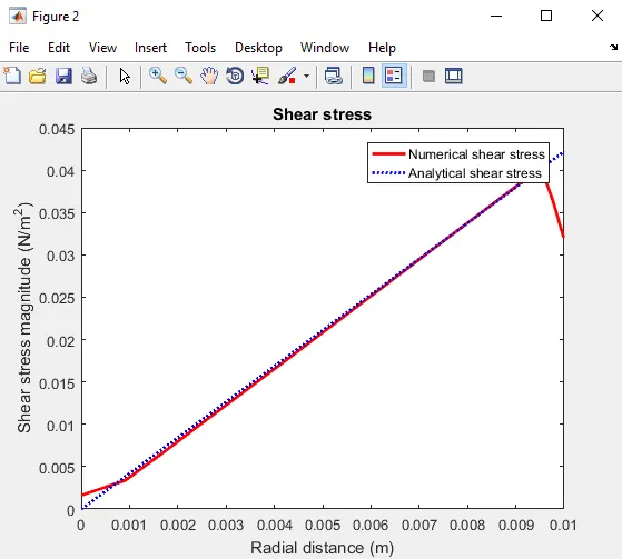
- The analytical values of velocity ,kinematic pressure & shear stress match with the numerical data from openfoam simulation .
- Velocity is maximum at the center of the pipe and decreases in magnitude as we measure velocity closer to the pipe wall ,this is because of the viscosity of the fluid medium inside the pipe .
- Pressure at the entire length of the fully developed flow region matches with our calculations .
- Shear stress plot displays a sudden dip in the graph after a gradual rise ,this is because of the meshing of the geometry .
However the analytical values and numerical values match one another .
Shear stress decreases as we approach the center of the pipe and gradually increases close to the wall . - Make sure that the CFL number does'nt exceed 0.5 by altering 'deltaT' in openfoam's controlDict file.