Week 3 - Solving second order ODEs

Aim:

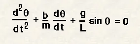
Objective is to write a program that solves the following ODE. This ODE represents the equation of motion of a simple pendulum with damping

In the above equation,

g = gravity in m/s^2,
L = length of the pendulum in m,
m = mass of the ball in kg,
b=damping coefficient.

use,
L=1 metre,
m=1 kg,
b=0.05,
g=9.81 m/s2
Simulate the motion between 0-20 sec, for angular displacement=0,angular velocity=3 rad/sec at time t=0.

Idealised pendulum:

An idealised pendulum is a swinging rigid body free to rotate about a fixed horizontal axis, consisting of a massless string of length "l" which suspends a pendulum bob of mass "m" .In addition a damping factor "b" may act due to friction at the pivot or due to air resistance or both together could dampen motion .
When a pendulum is displaced sideways from its equilibrium position it is subjected to a restoring force due to gravity that will accelerate it back towards the equilibrium position .
When released the restoring force acting on the pendulum's mass causes it to oscillate about the equilibrium position ,swinging back and forth .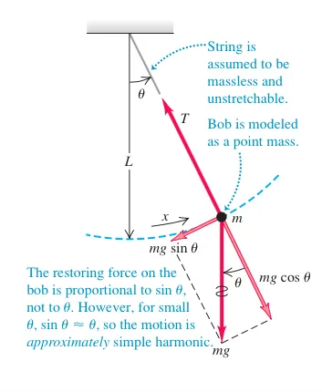

fig 1 : A pendulum with tangentail and radial force components.

To find the arc length of the pendulum ,
arc length('s' in radians)=Radius('r' in standard length)*theta(in radians)
`s=r*(theta)`
here ,r=l
`(ds)/dt = l*(d(theta))/dt`
`((d^2 s)/dt^2 ) = l*[(d^2(theta))/dt^2]`-------------------------(1)

Force ,'Fr' is countered by the tension due to the pivot and hence gets balanced.
so,'Ft' is the only force we will have to focus on for further calculation .

The forces acting on the pendulum bob are ,
i)Damping factor(b)
ii)Air resistance

so,
`F = -[mg*sin(theta)] - [b*(d(theta))/dt]`-----------------------------------(2)
The negative sign in '-[mg*sin(theta)]' is present to denote the direction of motion in negative direction.
The negative sign in '- [b*d(theta)/dt]' is present to denote that the damping causes resistance to motion of pendulum bob and hence reduces the force .

By Newton's 2nd law,
F = m*a
`F = m*((d^2.s)/dt^2)`-------------------------------(3)

here ,

Equating (1) & (2)
`m*((d^2.s)/dt^2) = - [mg*sin(theta)] - [b*(d(theta))/dt]`-------------------------------------(4)

Substituting (3) in (4),

`m*l*[(d^2(theta))/dt^2] = - [mg*sin(theta)] - [b*(d(theta))/dt]`
`(d^2(theta))/dt^2 = - [(g/l)*sin(theta)] - [{b/(m*l)}*(d(theta))/dt]`

from this equation we get ,

Function code:

• The code is written in MATLAB.
• The function starts with the keyword 'function' and declaration of output expected from the function, the function is named 'ode_func' and input arguments are passed.
• Theta1 is the first differential, theta2 is the transposed form of the equation shown above.
• The values obtained is converted into a column matrix with 2 columns.

function [dtheta_dt]=ode_func(t,theta,b,g,l,m)
theta1=theta(1)
theta2=theta(2)
dtheta1_dt=theta2
dtheta2_dt=-(b/m)*theta2-(g/l)*sin(theta1);
dtheta_dt=[dtheta1_dt; dtheta2_dt];
end

Main code:

• All the values important for calculation is first declared.
• Initial state of the system is angular displacement=0,angular velocity=3 rad/sec at time t=0.
• Time steps are created using linspace for 0 to 20 seconds.
• To call the function, we first name the outputs that we expect from the function.
  'ode45' is used to integrate the differential equations in the function to calculate 'theta' and 'angular velocity'.
• The outputs that is required is time values as a column matrix and results as a 2 column matrix where the first colum is the degree values that have been obtained by integrating the first differential, the 2nd column in the result matrix is the angular velocity.
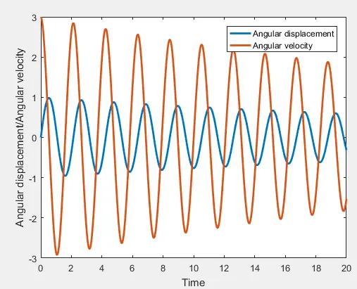
• The first plot shows the 'angular displacement' & 'angular velocity'.
• The second plot is an animation that stitches individual images to generate a movie file.
• The animation shows a pendulum bob oscillating (x1 & y1) about it's pivot (x0 & y0).
  The values of x1 and y1 change with each time step because of the change in the angular displacement.
• Further the code generates a movie file which shows the animation.

clear all
close all
clc

b=0.05;
g=9.81;
l=1;
m=1;

%initial condition
theta_0=[0;3];

%time points
t_span=linspace(0,20,500);

%solve ODE
[t, results]=ode45(@(t,theta) ode_func(t, theta, b, g, l, m),t_span,theta_0);

plot(t, results(:,1),'linewidth',2)
hold on
plot(t, results(:,2),'linewidth',2)
legend('Angular displacement','Angular velocity')
ylabel('Angular displacement/Angular velocity')
xlabel('Time')


figure(2)
ct=1;
for i=1:length(t_span)
    
% the point node,pivot
    h0=0;
    v0=0;
% the position of the pendulum bob 
    h1=sin(results(i,1));
    v1=-cos(results(i,1));
    plot([h0 h1],[v0 v1],[-0.5 0.5],[0 0],'linewidth',3)
    hold on   
% pendulum bob in animation
    plot(h1,v1,'marker','o','markerSize',20,'markerFacecolor','r')
    axis([-1.5 1.5 -1.5 0.5])
    grid on 
    pause(0.001)
% generation of multiple frames
    M(ct)=getframe(gcf);
    ct=ct+1;
    hold off
end

%movie(M)
videofile=VideoWriter('pendulum_function.avi','Uncompressed AVI');
open(videofile)
writeVideo(videofile,M)
close(videofile)

Results:

Animated video:

Animation