Week 5.2 - Literature review: ODE Stability

Literature review on stability of ODE :

When does a ODE become unstable?

Section 1 : Equilibria are not always stable. Since stable and unstable equilibria play quite different roles in the dynamics of a system, it is useful to be able to classify equilibrium points based on their stability. Suppose that we have a set of autonomous ordinary differential equations, written in vector form:

`dotx=f(x)`

Suppose that x is an equilibrium point. By definition, f(x) =0. Now suppose that we take a multivariate Taylor expansion of the righthand side of our differential equation:

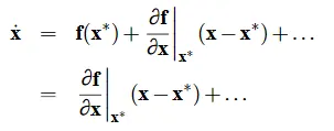
The partial derivative in the above equation is to be interpreted as the Jacobian matrix. If the components of the state vector x are (x1;x2;….;xn)and the components of the rate vector f are (f1;f2; …;fn), then the Jacobian is

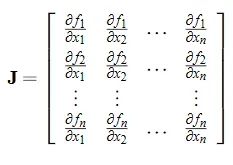
Now define `delx=x-x^(star)`
Taking a derivative of this definition, weget `del^(')x= x'`. If `delx` is small, then only the first term in equation 2 is significant since the higher terms involve powers of our small displacement from equilibrium. If we want to know how trajectories behave near the equilibrium point, e.g.whether they move toward or away from the equilibrium point, it should therefore be good enough to keep just this term 1 Then we have

`del^(')x=J^(star)delx`

Where `J^(star)` is the Jacobian evaluated at the equilibrium point.
The matrix `J^(star)` is a constant, so this is just a linear differential equation. According to the theory of linear differential equations, the solution can be written as a superposition of terms of the form `e^(lambda_jt)` where {`lambda_j`} is the set of eigen values of the Jacobian .

The eigen values of the Jacobian are, in general, complex numbers.
Let `lambda_j=mu_j+i* νj`, where `mu_j` and `v_j` are, respectively, the real and imaginary parts of the eigenvalue. Each of the exponential terms in the expansion can therefore be written

`e^(λ_jt)=e^(mu_jt)*e^(i*ν_jt)`

The complex exponential in turn can be written `e^(i*ν_jt) = cos(ν_jt) +i*sin(ν_jt)`

The complex part of the eigenvalue therefore only contributes an oscillatory component to the solution. It’s the real part that matters :
If `mu_j>0` for any j , `e^(mu_jt)` grows with time, which means that trajectories will tend to move away from the equilibrium point.

In addition to having a stable problem, i.e., a problem for which small changes in the initial conditions elicit only small changes in the solution, there are two basic notions of numerical stability. The first notion of stability is concerned with the behavior of the numerical solution for a fixed value t > 0 as `h->0`.

Numerical IVP solver is zero stable if small perturbations in the initial conditions do not cause the numerical approximation to diverge away from the true solution provided the true solution of the initial value problem is bounded.

Stability is concerned with the behavior of the solution as `t->infty`with a fixed stepsize h. This notion of stability is often referred to as absolute stability, and it is important when dealing with stiff ODEs. An absolutely stable numerical method is one for which the numerical solution of a stable problem behaves also in this controlled fashion.

Model Problem: For `lambdainR` we consider the family of scalar linear initial value problems

`y′(t) =lambda*y(t), t∈[0,T]`

`y(0) =y_0`

The solution of this problem is given by

`y(t) = y_0e^(lambdat)`

Now we take the same differential equation, but with perturbed initial condition

`y_delta(0) = y_0 + delta``lambda > 0`

Then the general solution still is `y_delta(t) = ce^(lambdat)`. However, the initial condition now implies

`y_delta(t) = (y_0 + delta)e^(lambdat)`

Therefore, if `lambda<=0`, a small change in the initial condition causes only a small change in the solution and therefore the problem is a stable problem. However, if , then large changes in the solution will occur (even for small perturbations of the initial condition), and the problem is unstable. Therefore, when studying the stability of numerical methods we will consider the model problem for `lambda<=0` only. Even though we will study only stability with respect to the model problem, it can be shown that the results of this analysis also apply to other linear (and some nonlinear) problems.

Section 2 : Euler's method :

We study how Euler’s method behaves for the stable model problem above, i.e., in the case `lambda <= 0`. Since `f (t, y) = lambday(t)` Euler’s method states that

`y_(n+1) = y_n + hf (t_n, y_n)`

`= y_n + h*lambday_n`

`= (1 + lambdah)y_n.`

Therefore, by induction,

`y_n = (1 + lambdah)^ny_0`

Since the exact problem has an exponentially decaying solution for λ < 0, a stable numerical method should exhibit the same behavior. Therefore, in order to ensure stability of Euler’s method we need that the so-called growth factor |1 + λh|< 1. For real λ < 0 this is equivalent to

`−2< hlambda <0 harr h <−2/lambda.`

Thus, Euler’s method is only conditionally stable, i.e., the step size has to be chosen sufficiently small to ensure stability.

Section 3 : Implicit or backward Euler method :

Expand the function Y(x) as a linear Taylor polynomial about `x_(n+1)` :

`Y(x) =Y(x_(n+1)) + (x−x_(n+1))Y′(x_(n+1)) +1/2*(x−x_(n+1))^2*Y′′(zeta_n)`

with `zetan` in between x & `x_(n+1)`.The Backward euler method is obtained by dropping the truncation error :

`Y_(n+1)=Y(x_n)+hY'(x_(n+1))-1/2h^2Y''(zeta_n)`

=`Y(x_n)+hf(x_(n+1),Y(x_(n+1)))-1/2h^2Y''(zeta_n)`

with `zeta_n`between `x_n` and `x_(n+1)`.The backward Euer method is obtained by dropping the truncation error .

`y_(n+1)=y_n+hf(x_(n+1),y_(n+1)),` `n=0,1.....`

`y_0=Y_0`

The truncation is essentially of the same size as for Euler's mathod but of opposite sign .

Apply the backward Euler method to the model problem

`Y'(x)=lambdaY(x),` `x>=0,Y(0)=1`

This yields

`y_(n+1)=y_n+h*lambda_(n+1)`

`y_(n+1)=1/(1-hlambda)*y_n` `n=0,1....`

with `y_0=1`

By induction ,
`y_n=(1/(1-hlambda))^n` , `n=0,1....`

We want to know when `y_n->0` as `n->infty` .

This will be true if `|1/(1-hlambda)|<1`

The hypothesis that `lamda<0` is suffecient to show this is true ,regardless of the size of the stepsize h .Thus the backward Euler method is an A.

If `|λ|` is quite large, then h must be correspondingly small. Usually the truncation error does not require such a small value of h ; it is needed only for stability.

Code details :

Assumed equation : `dy/dt=-10000y-e^(-t)`

Explicit condition : Euler method

`(y^(n+1)-y^n)/(Deltat)=-10000y^n-e^(-t)`

`y^(n+1)=y^n-(10000y^n-e^(-t))`

Here, n = Old value & n+1 = New value

Implicit equation : Backward difference auler method

`(y^(n)-y^(n-1))/(Deltat)=10000y^n-e^(-t)`

`y^n=(-10000y^n-e^(-t))Deltat+y^(n-1)`

`y^n-(-10000y^n-e^(-t))Deltat=y^(n-1)`

`y^n+(10000y^n+e^(-t))Deltat=y^(n-1)`

`y^n(1+10000Deltat)+e^(-t)Deltat=y^(n-1)`

`y^n=(y^(n-1)-e^(-t)Deltat)/(1+10000Deltat)`

Here, n-1 = Old value & n = New value

Code :

import numpy as np
import matplotlib.pyplot as plt

def explicit_euler(total_t,dt):

	t=np.arange(0,total_t,dt)
	y=np.zeros(len(t))

	for i in range(1,len(t)):
		y[i]=y[i-1]+dt*(-10000*y[i-1]-np.exp(-t[i-1]))			    
	return [t,y]

def implicit_euler(total_t,dt):

	t=np.arange(0,total_t,dt)
	y=np.zeros(len(t))

	for i in range(1,len(t)):
		y[i]=(y[i-1]-np.exp(-t[i-1])*dt)/(1+10000*dt)				
	return [t,y]

def analytical(total_t,dt):

	t=np.arange(0,total_t,dt)
	y=np.zeros(len(t))

	for i in range(1,len(t)):
		y[i]=np.exp(-10000*t[i])*(1-np.exp(9999*t[i]))/9999
	return y


total_t=0.1
dt=1e-4 		
										
t,y_explicit=explicit_euler(total_t,dt)
t,y_implicit=implicit_euler(total_t,dt)
y_analytical=analytical(total_t,dt)
plt.plot(t,y_explicit,color='blue')
plt.plot(t,y_implicit,color='black')
plt.plot(t,y_analytical,color='red')
plt.legend(['Explicit','Implicit','Analytical'])
plt.xlabel('t')
plt.ylabel('y')
plt.show()

Plots :

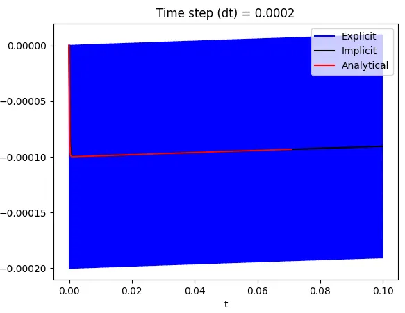
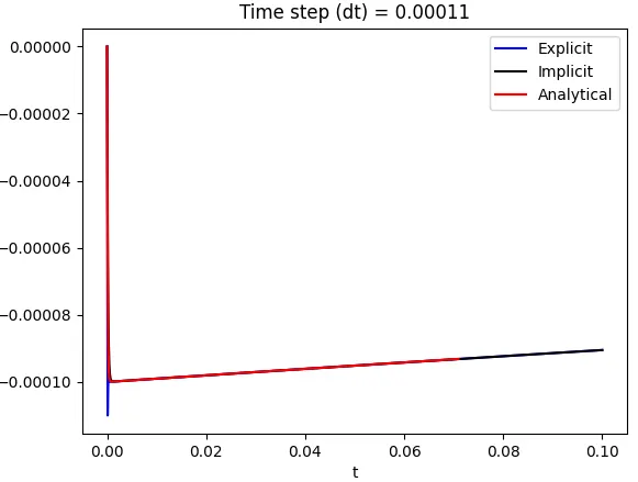
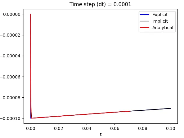
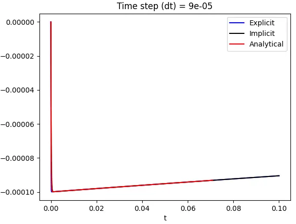
From the above plots we can observe that the analytical and implicit lines overlap on one another at all time steps 'dt' but the explicit solution is very sensitive to the change in 'dt'.
Once the oscillation arises then as we increase 'dt' the oscillations increases more and more .

How does stability affect engineering simulations?

In engineering simulations stability is a very serious issue and the explicit schemes require more quantities for it to maintain stability .We can see this from the above exercise .However ,this is not applicable for implicit schemes .When there is oscillations in a system of equation then the oscillation grows in magnitude until the solution completely blows up as shown in plot 1 .Also note that the deviation of explicit just starts at time step 0.00011.

Can stability condition be derived for all types of problems?

In Section I there is suffecient information about when an equation can attain equilibria .
By using suffecient modifications in the approximation we can attain stability as seen from above exercise ,the difference between implicit backward euler and explicit euler method is visible and proves that by modifying the equation we can attain stability for a particular problem .