Week 3 - External flow simulation over an Ahmed body.
AIM:
To simulate flow over ahmed body & to address the below given tasks.
1. Describe Ahmed body & its importance.
2. Explain the negative pressure in wake.
3. Explain significance of the point of seperation.
Expected results:
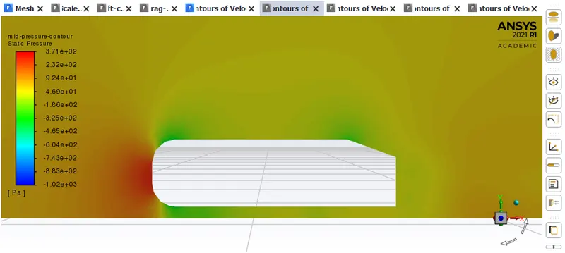
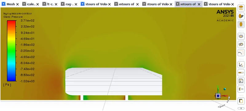
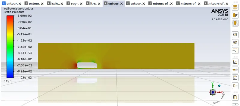
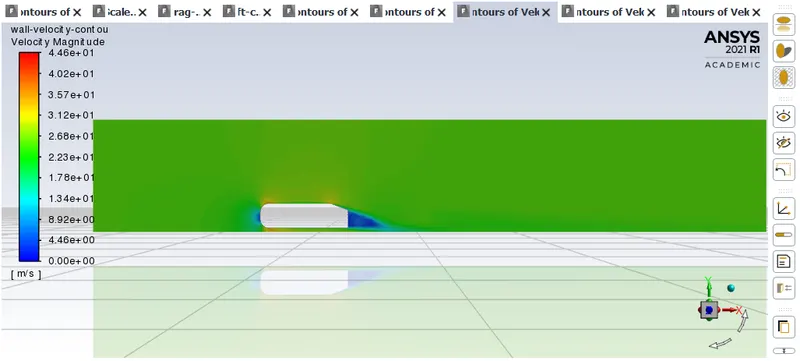
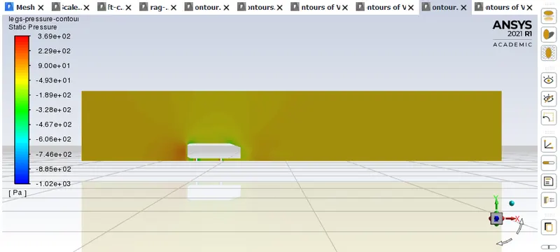
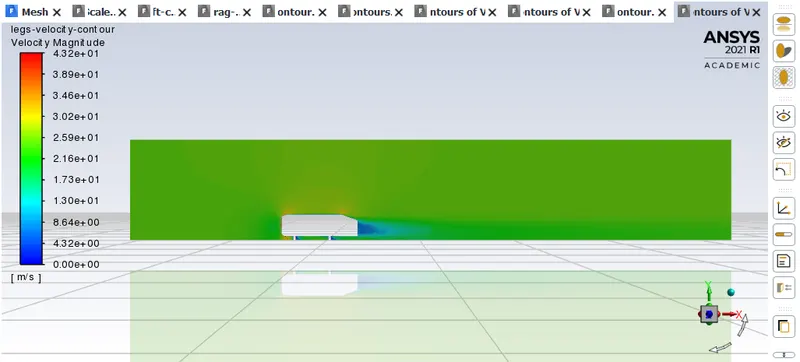
1. Velocity & pressure contour of the Ahmed body.
2. Cd for a refined case. (for velocity = 25m/s, Cd = 0.33)
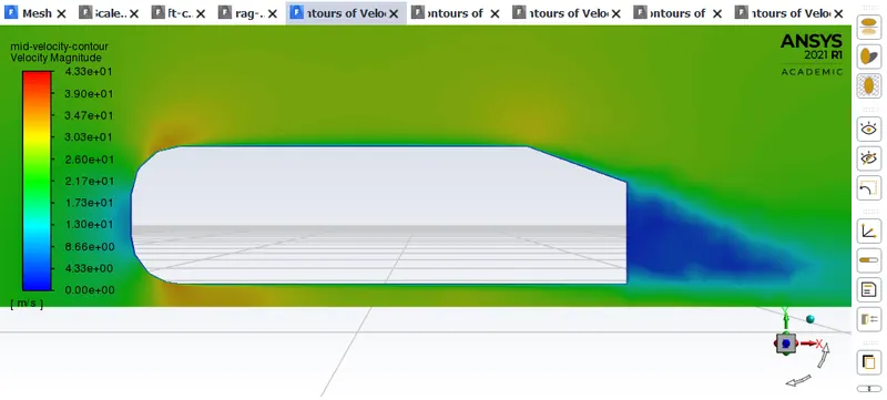
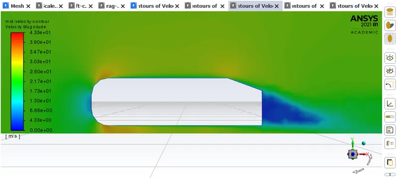
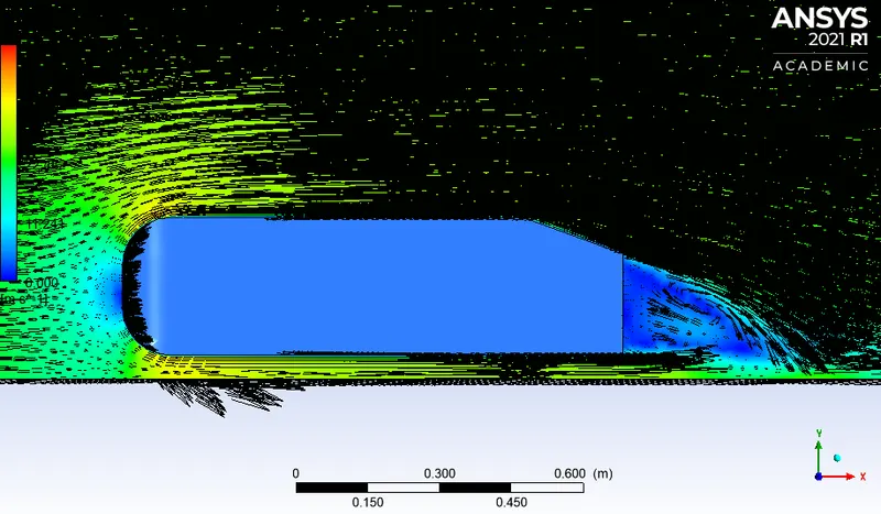
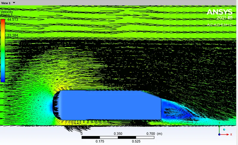
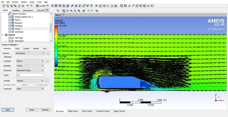
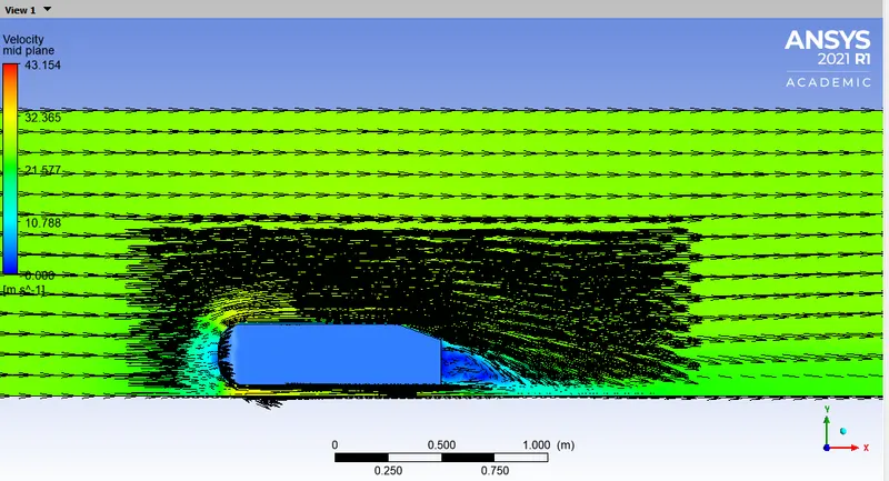
3. Vector plot must show wake region.
4. With grid dependency test provide Cd & Cl for each case.
Note:
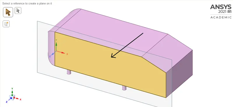
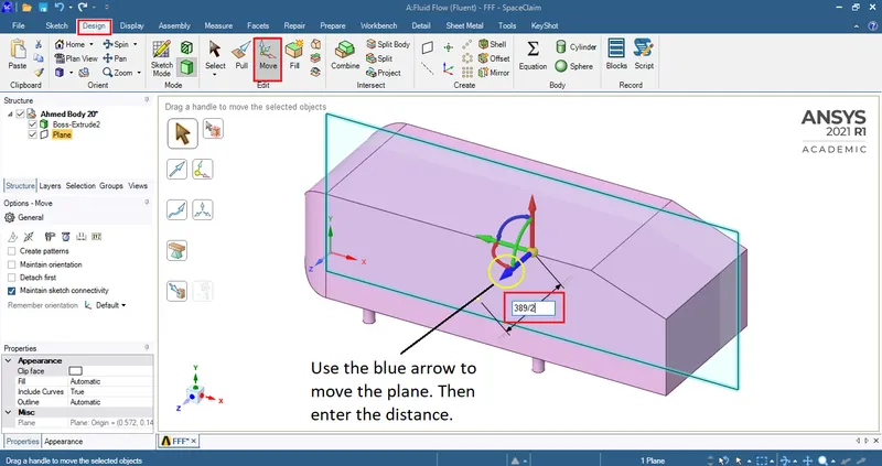
1. Since the ahmed body is symmetric, run the simulatoion by considering only half body. Doing this would increase the cell count and would make the mesh finer.
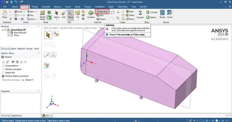
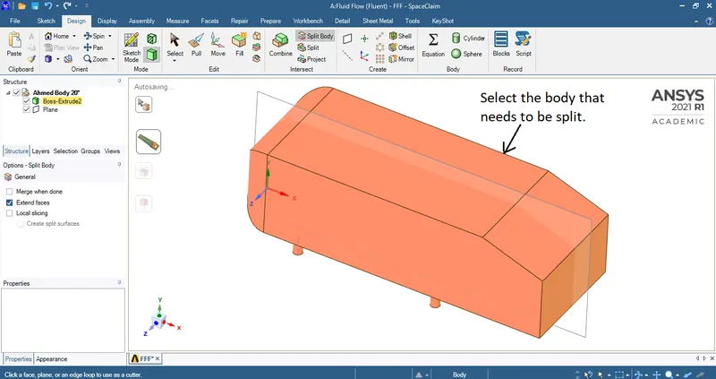
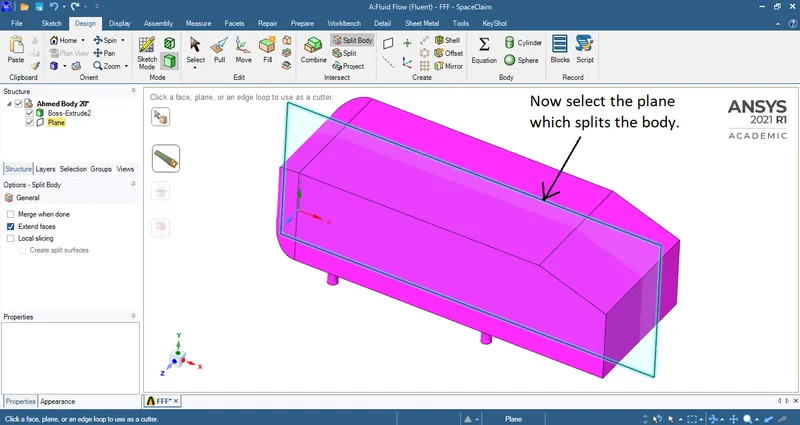
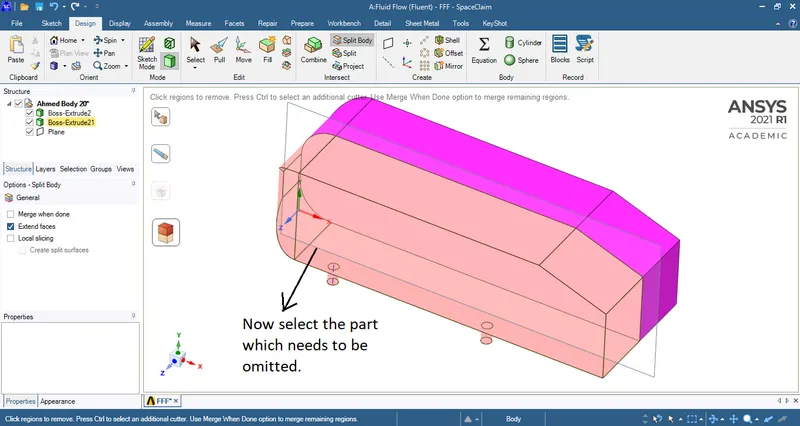
2. Use split body command in spaceclaim & use symmetry boundary condition.
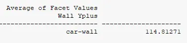
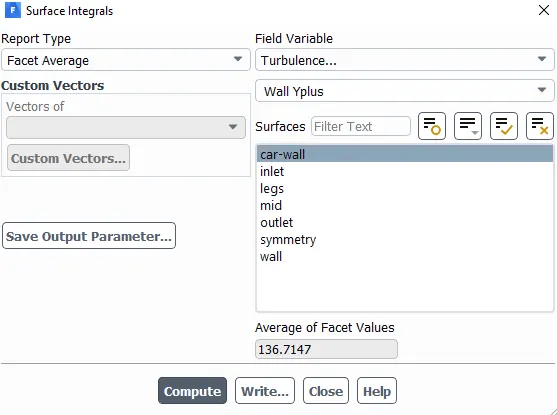
3. Maintaining an appropriate y+ value will give correct Cd value.
Theory:
Reynold's number:
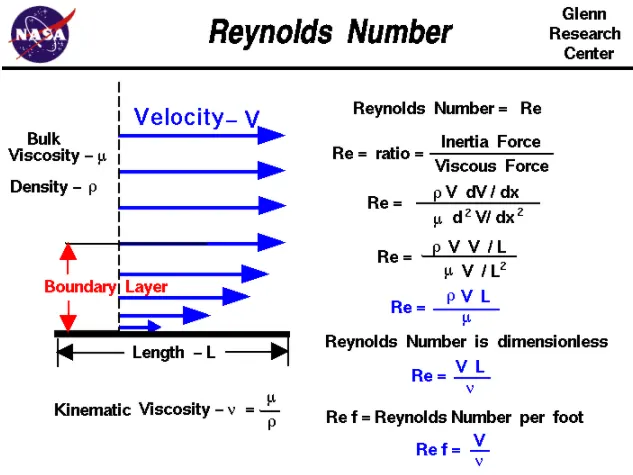
Boundary layer for flow over a flat plate:
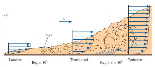
Transition of the laminar boundary layer on a flat plate into a fully turbulent boundary layer (not to scale).
The vertical scale has been greatly exaggerated, and the horizontal scale has been shortened (in reality, since Rex, transition ≅ 30 times Rex, critical, the transitional region is much longer than indicated in the figure).
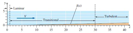
Thickness of the boundary layer on a flat plate, drawn to scale. Laminar, transitional, and turbulent regions are indicated for the case of a smooth wall with calm free-stream conditions.
In real-life engineering flows, transition to turbulent flow usually occurs more abruptly and much earlier (at a lower value of `Re_x`) than the values given for a smooth flat plate with a calm free stream. Factors such as roughness along the surface, free-stream disturbances, acoustic noise, flow unsteadiness, vibrations, and curvature of the wall contribute to an earlier transition location. Because of this, an engineering critical Reynolds number of `Re_(x, cr)= 5*10^5` is often used to determine whether a boundary layer is most likely laminar (`Re_x` < `Re_(x, cr)`) or most likely turbulent (`Re_x` > `Re_(x, cr)`).
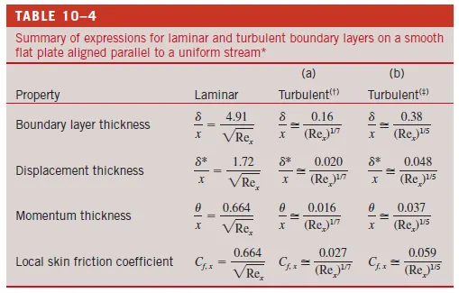
* Laminar values are exact and are listed to three significant digits, but turbulent values are listed to only two significant digits due to the large uncertainty affiliated with all turbulent flow fields.
† Obtained from one-seventh-power law.
‡ Obtained from one-seventh-power law combined with empirical data for turbulent flow through smooth pipes.
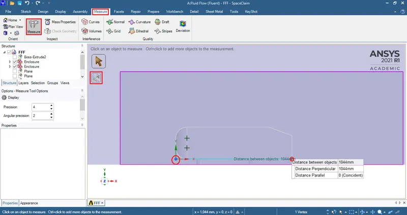
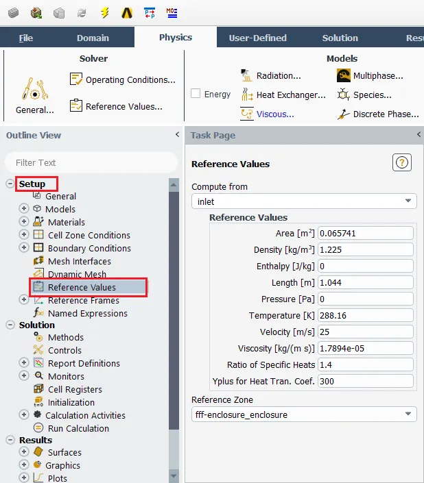
Since the characteristic length has been found to be 1044mm(1.044m) the Reynold's number of the flow can be calculated.
Other qualtities that are known:
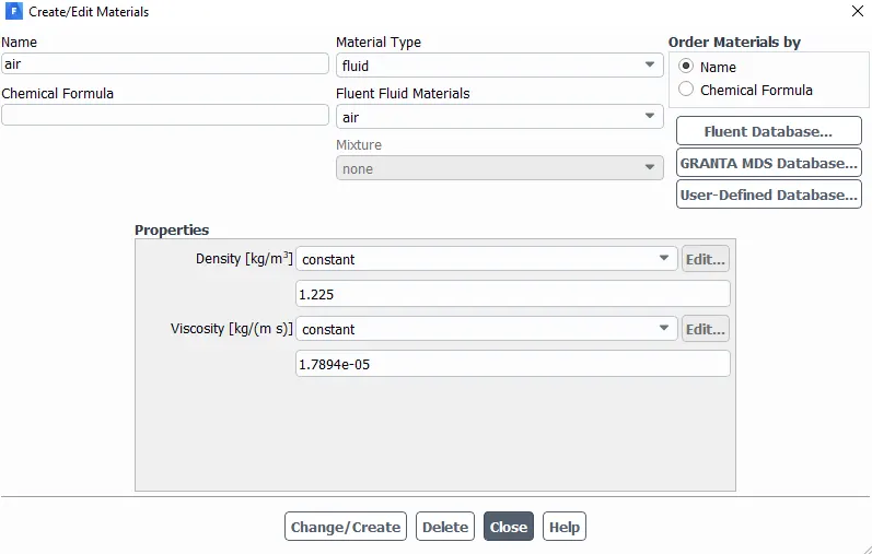
Properties of fluid:
Fluid medium: Air
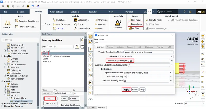
V=Velocity=25m/s
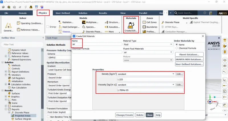
`rho`=Density=`1.225(kg)/m^3`
`mu`=Dynamic viscosity=`1.7894*10^(-5)(kg)/(ms)`
Reynold's number = `(rhoVL)/mu`
=`(1.225(kg)/(m^3)*1.044m*25m/s)/((1.7894*10^(-5))(kg)/(ms))`
=`1786772.102`
For such a high Reynold's number a turbulent model has to be used.
Geometry description:
Ahmed body:
The Ahmed Body was first created by S.R. Ahmed in his research “Some Salient Features of the Time-Averaged Ground Vehicle Wake” in 1984. Since then, it has become a benchmark for aerodynamic simulation tools. The simple geometrical shape has a length of 1.044 meters, height of 0.288 meters, and a width of 0.389 meters. It also has 0.5-meter cylindrical legs attached to the bottom of the body and the rear surface has a slant that falls off at 40 degrees.
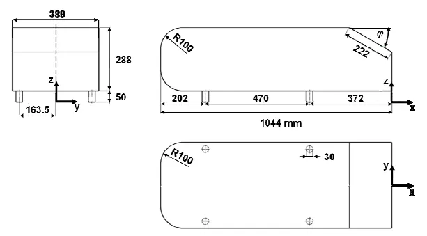
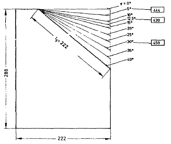
Selection of the configuration used in this study was governed by the requirement that it should generate the essential features of a real vehicle flow field, with the exception of that due to rotating wheels, engine and passenger compartment flow, rough underside and surface projections. It was conjectured that the model chosen should generate: a strong three-dimensional displacement flow in front, relatively uniform flow in the middle, and a large structured wake at the rear. The wind tunnel model, with an overall length of 1.044 m had a length: width: height ratio of 3.36 : 1.37 : 1. It consisted of three parts;
a fore body,
a mid section and
a rear end.
Edges of the fore body were rounded, as indicated above to achieve a separation free flow over its surface. Middle section was a box shaped sharp edged body with a rectangular cross section.
Importance of Ahmed body:
As the burning of fossil fuels becomes a more pressing issue, manufacturers are introducing more fuel efficient cars to the market. One main contributor to fuel burn is the car’s aerodynamic drag. Complexly shaped, cars are very challenging to model and it’s difficult to quantify the aerodynamic drag computationally. The Ahmed body is a benchmark model widely used in the automotive industry for validating simulation tools. The Ahmed body shape is simple enough to model, while maintaining car-like geometry features.
The drag coefficient quantifies the resistance of an object in a fluid environment. It is not an absolute constant for a body’s shape because it varies with the speed and direction of flow, object shape and size, and the density and viscosity of the fluid. The lower the drag coefficient of an object, the less aerodynamic or hydrodynamic drag occurs. In terms of a car, the lower the drag coefficient, the more efficient the car is. As well as affecting the top speed of a vehicle, the drag coefficient also affects the handling. Cars with a low drag coefficient are sought after, but decreasing the drag drastically can reduce the downforce and lead to loss in road traction and a higher chance of car accidents.
Most cars have an average drag coefficient of between 0.30 and 0.35. Boxy cars have a higher number, like the HUMMER® H2 vehicle at 0.57, while more streamlined and agile cars have a lower number, like the Mercedes-Benz® C-Class® vehicle at 0.24. Again, this is just an average measurement. The exact drag coefficient of a car varies with the Reynolds number and various other factors.
There are certain ways to modify a car to optimize its aerodynamics and decrease the drag coefficient. To streamline the exterior, you can remove certain aftermarket items such as the roof rack, mud flaps, spoilers, and radio antenna. Professional car racers also take off their windshield wipers and side mirrors, but this isn’t recommended for the average driver! You can also add wheel covers, a partial grille block, an under tray, fender skirts, and a modified front bumper to improve the drag coefficient and make your car stand out in the process.
Baseline setup:
1) K-epsilon(standard): Transient
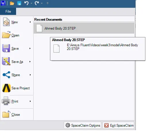
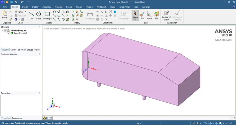
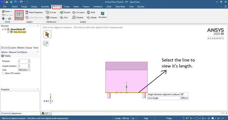
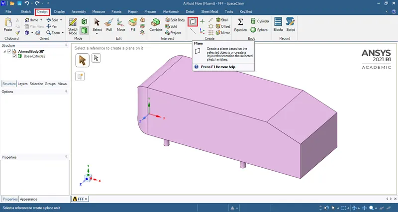
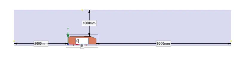
Side view:
Top view:
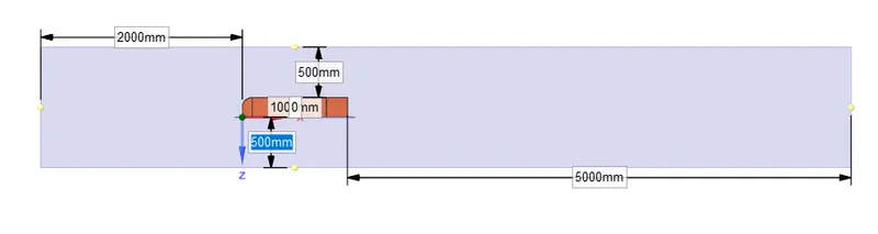
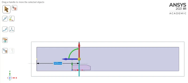
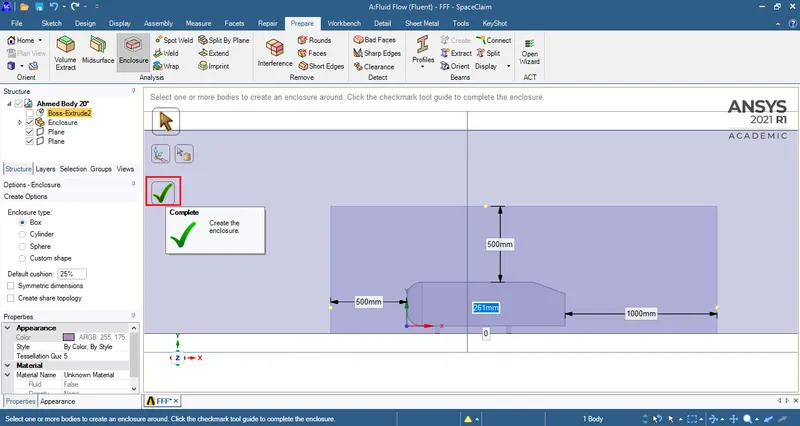
To finish click the green tick.
Creating a plane to view material hashing in the cross sectional view.
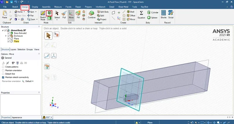
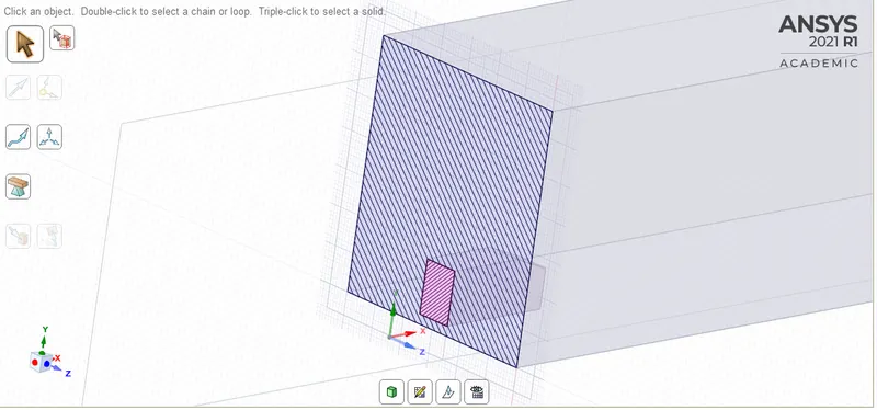
Since the domain around the 'Ahmed body' is required for simulation the inner hashing has to be hidden by unchecking it from under the 'Structure' on the left hand side.
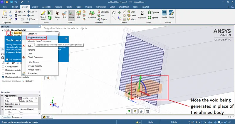
In addition to this the 'Ahmed body' has to be excluded during simulation and hence must use 'supress for physics' option.
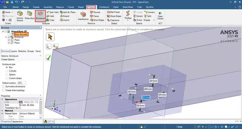
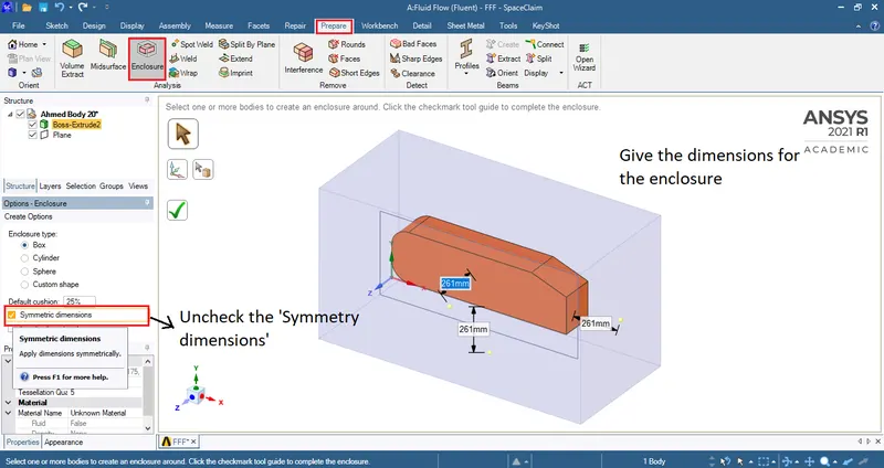
Enter the dimensions for the newly formed enclosure.
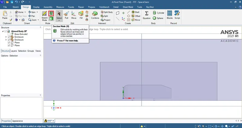
After selecting the Selection mode hit on the plane to view the hashings.
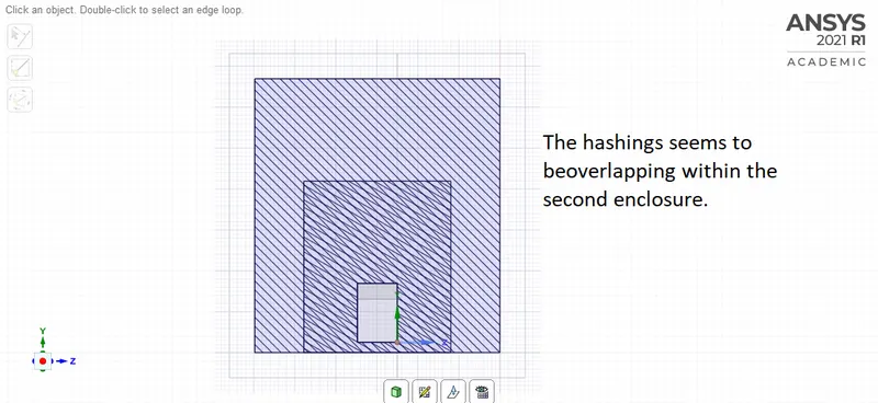
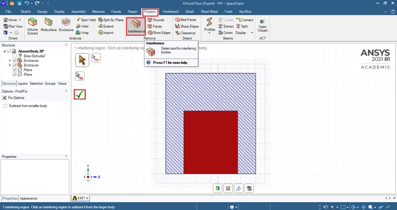
When the green tick mark is clicked, the interferanceissue will be solved resulting in a clear distinction between the hashings of different enclosures.
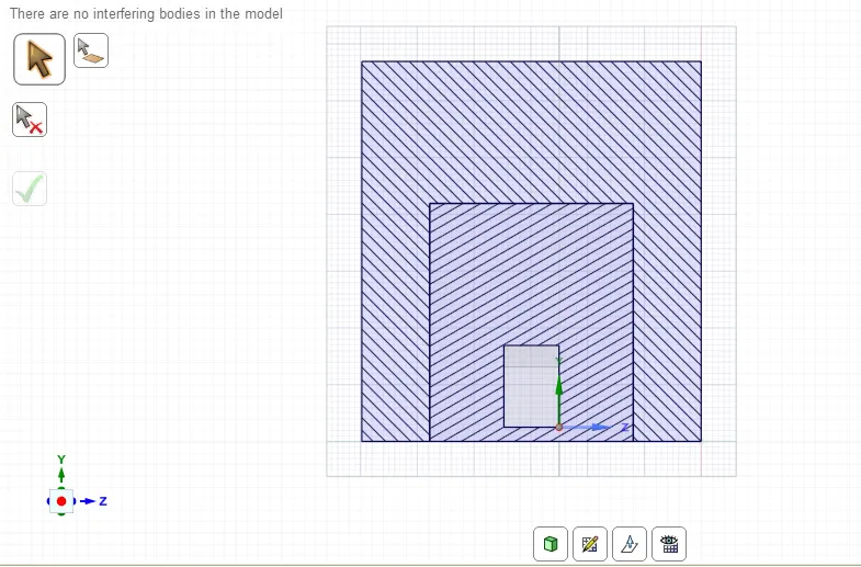
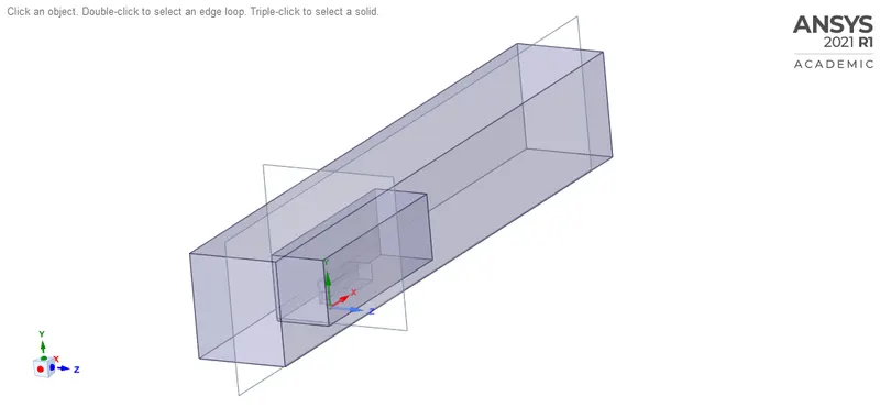
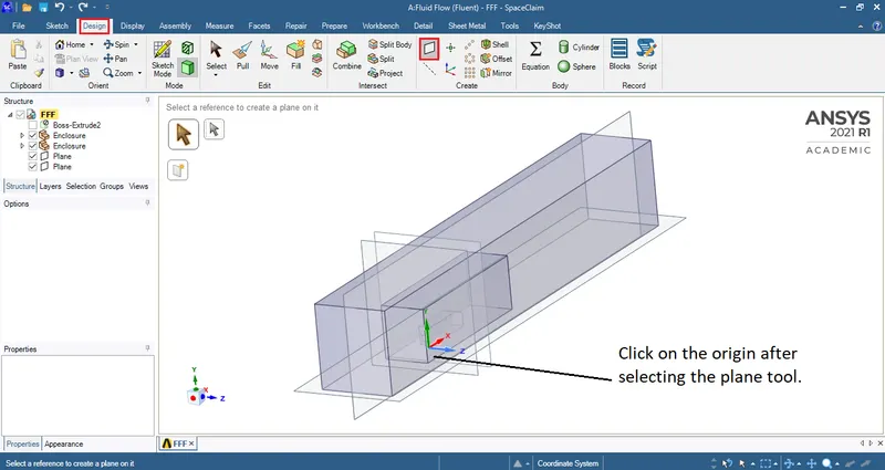
Error!
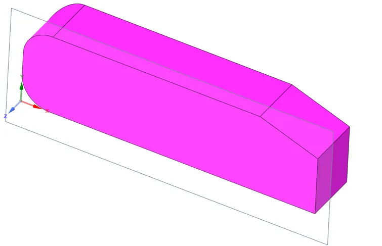
Here the 'Ahmed body' which is symmetrical from nose to tail has been cut up in half to generate finer cells. Since only half of the body will be analysed the number of large sized cells required will reduce and the number of small and fine cells increases.
The issue at hand now is the enclosure has been created for the whole body.
The corrective measure to this issue would be to split and delete the excess enclosures.
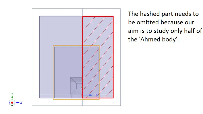
Body split command can be used to delete the excess enclosure.
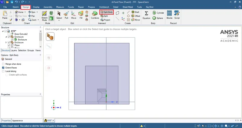
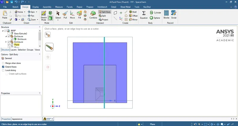
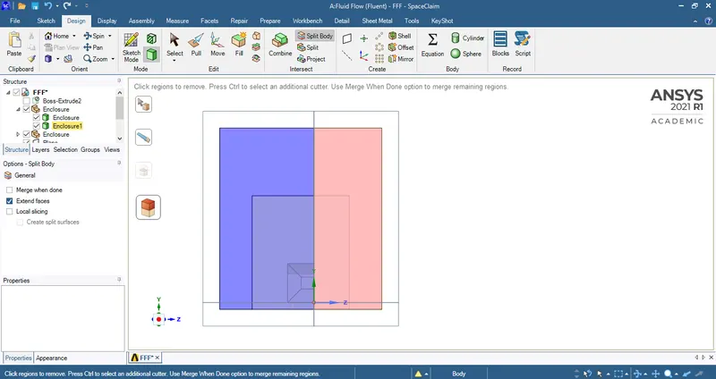
Follow the same steps to delete the excess from the inner enclosure.
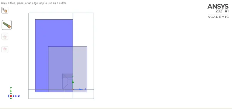
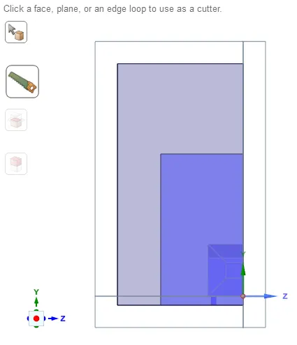
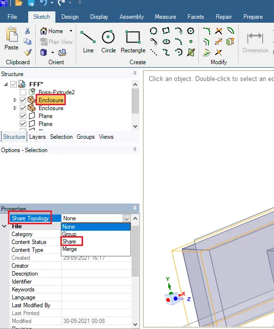
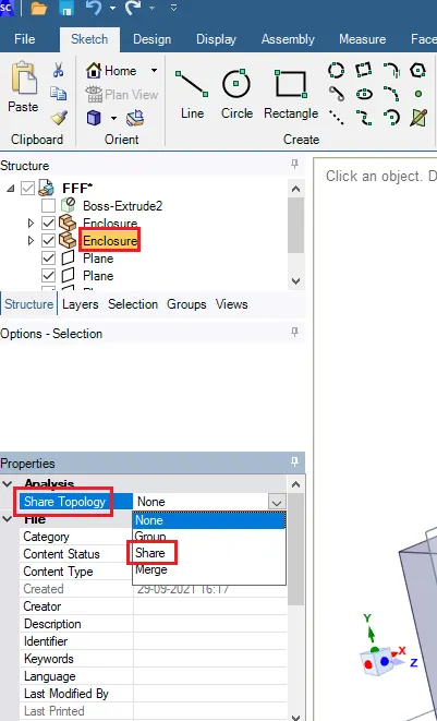
This ensures that information exchange happens between the 2 enclosures.
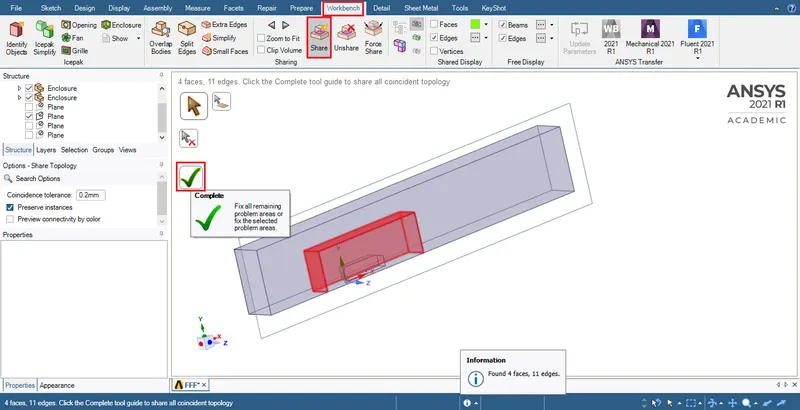
Just to be sure about sharing topology go to workbench and do as shown above.
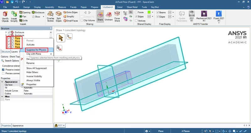
Close the spaceclaim window and open the meshing interface.
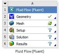
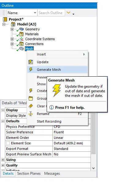
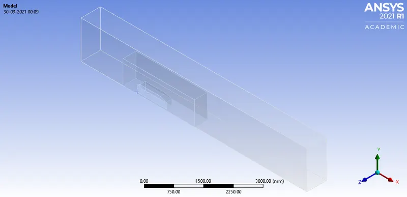
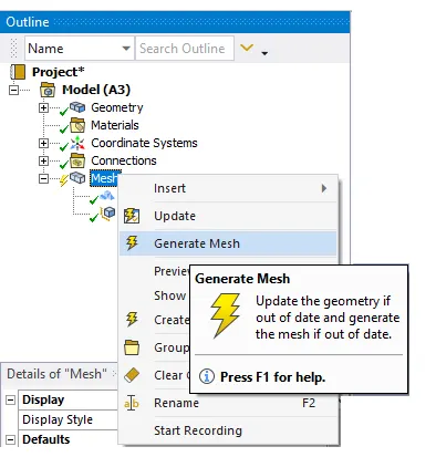
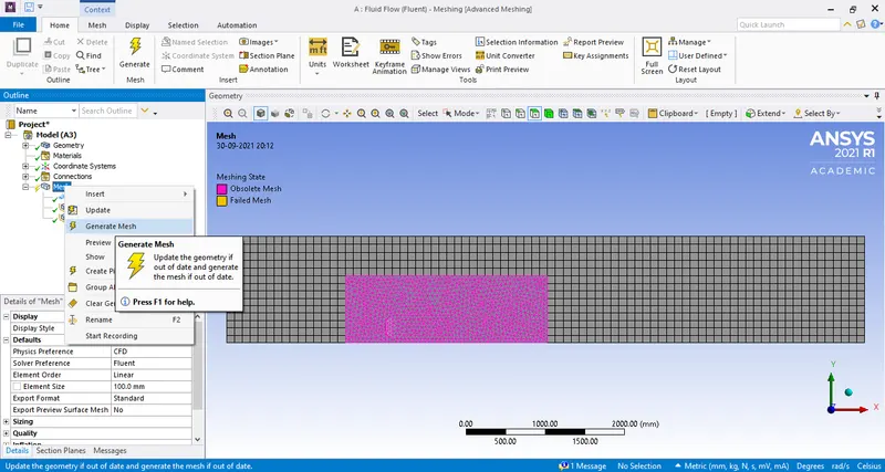
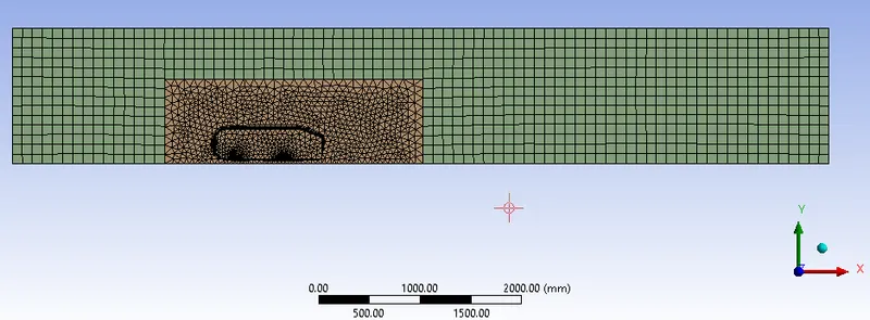
To use hexahedral mesh which would prefectly fit the cuboidal enclosure.
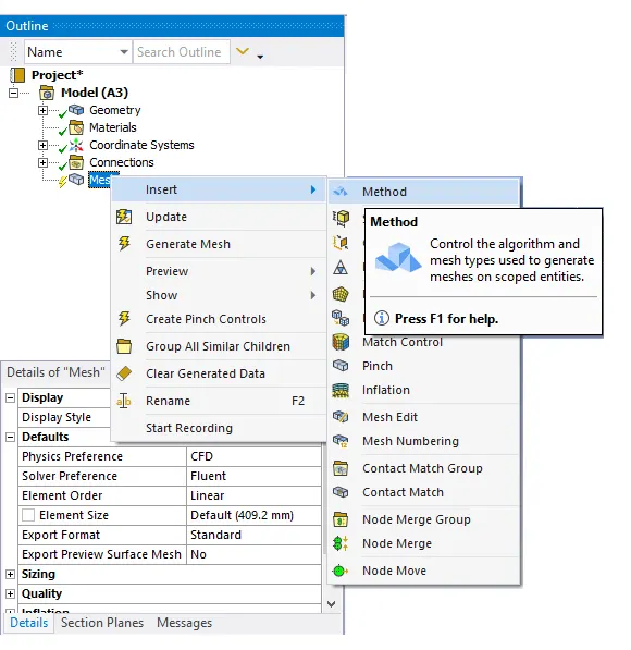
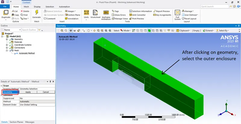
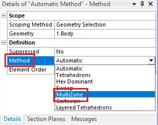
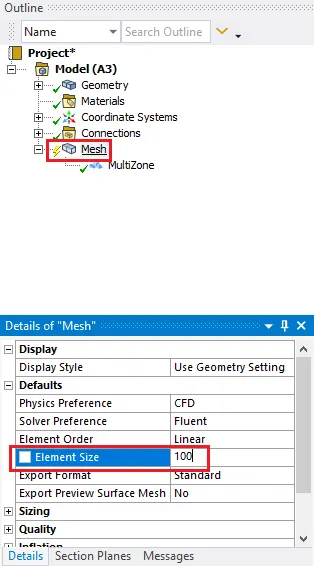
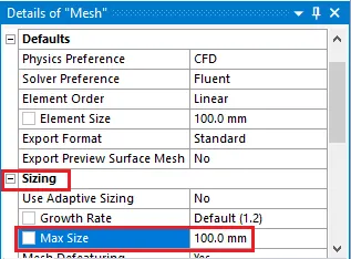
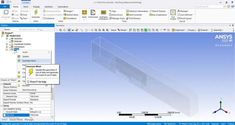
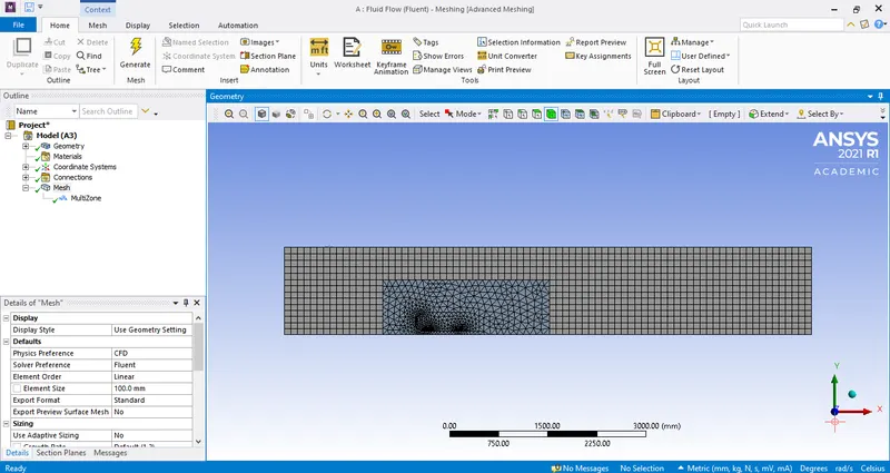
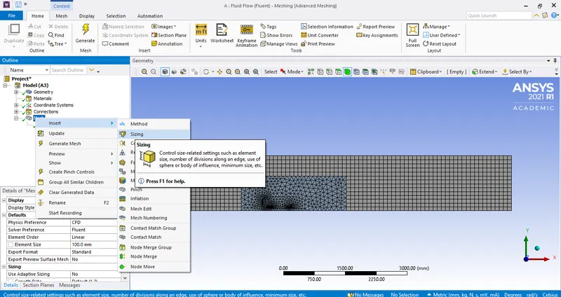
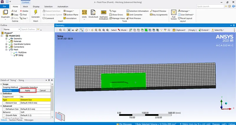
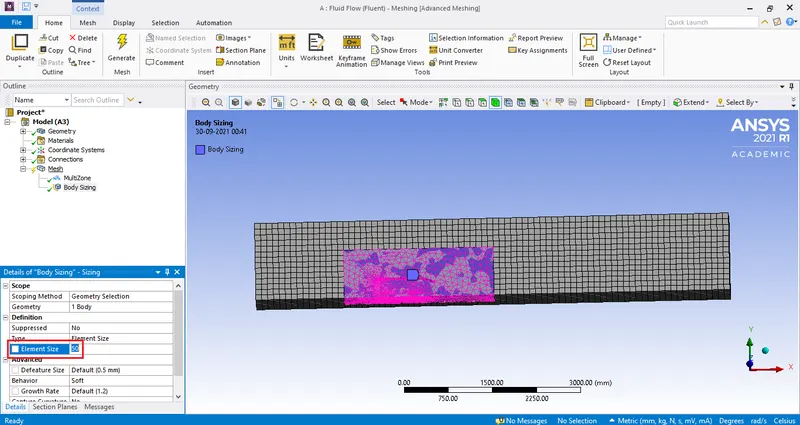
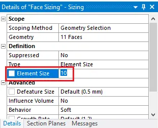
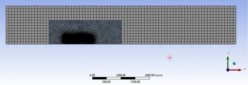
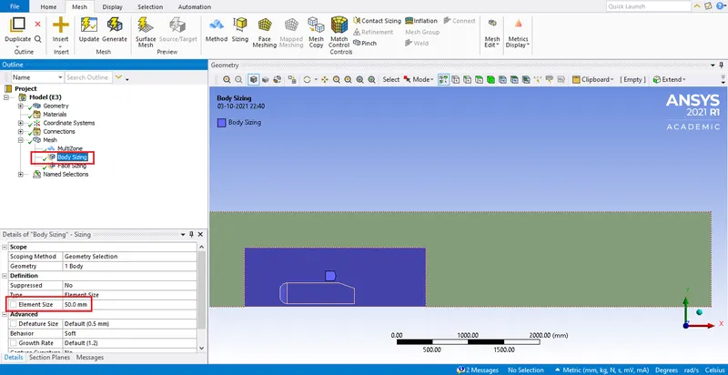
Choosing a smaller mesh size for the inner enclosure.
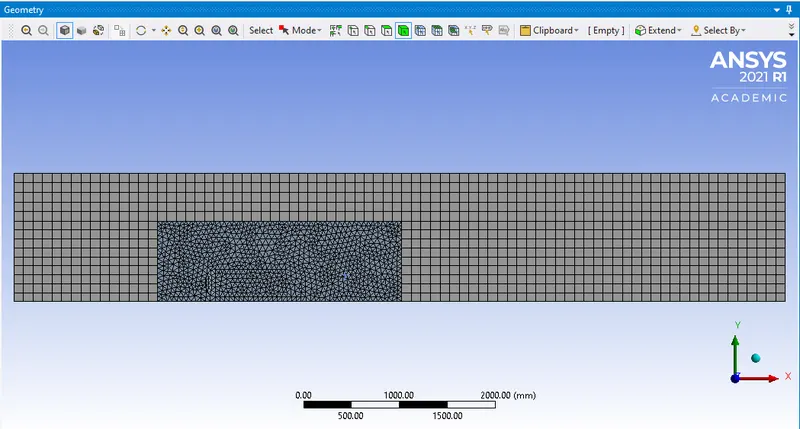
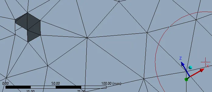
At the bottom we see polygonal profile for the circles, so this calls for further mesh refinement.
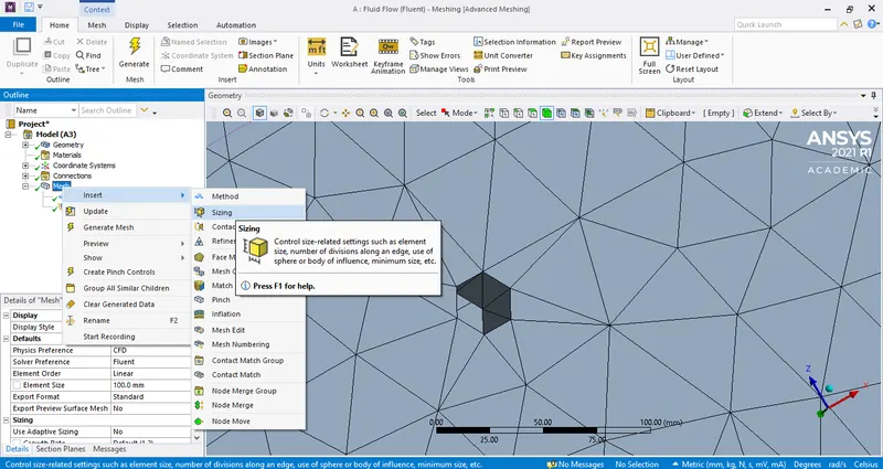
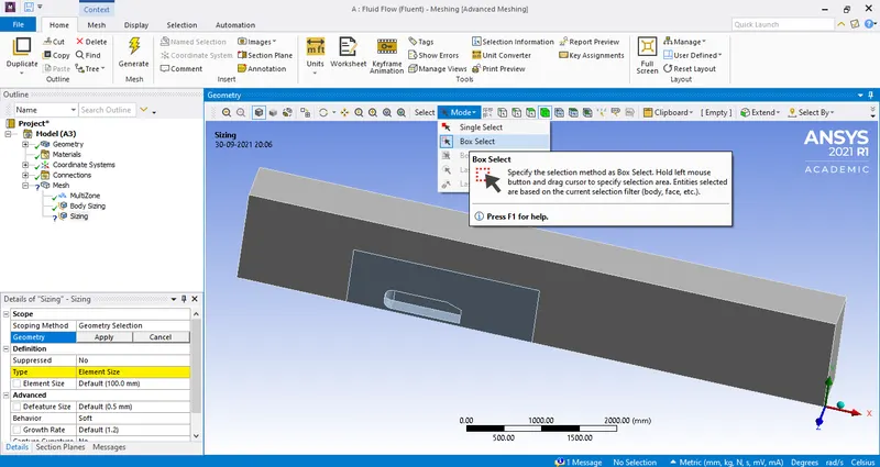
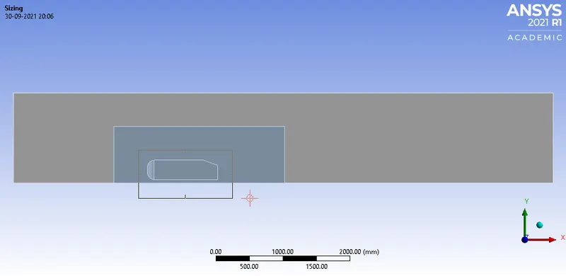
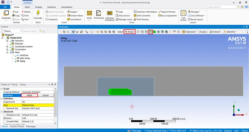
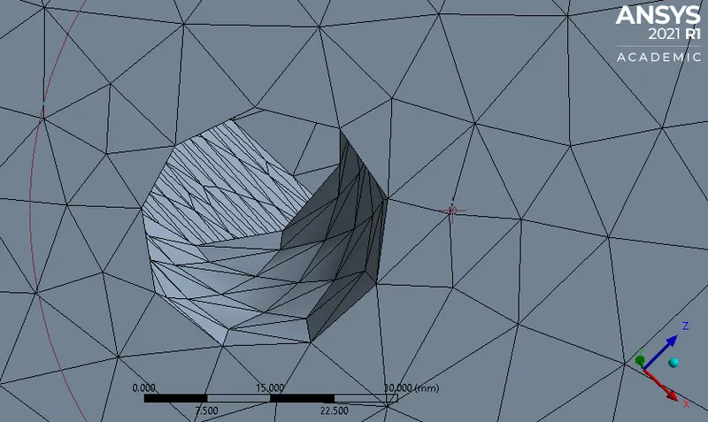
The contours still resemble a polygon so an alternate operation must be made.
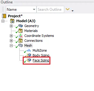
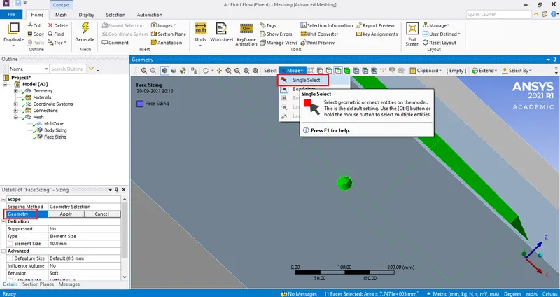
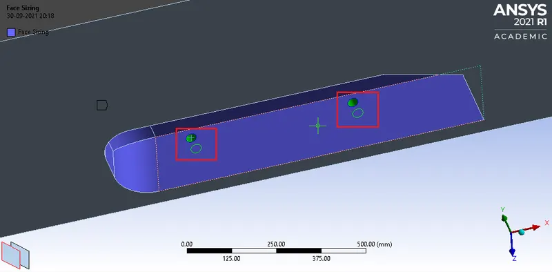
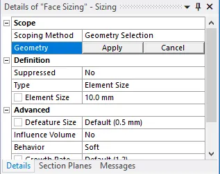
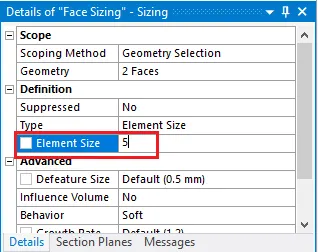
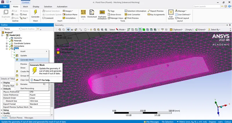
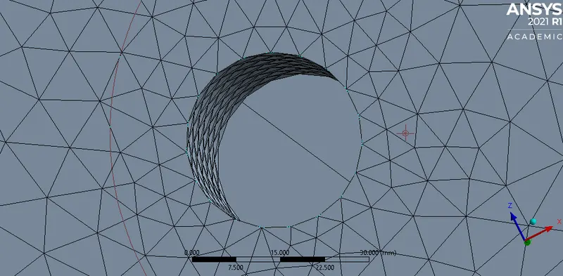
Now the contours resemble a circle.
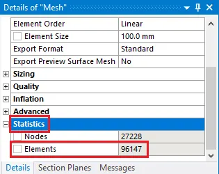
Now the mesh can be optimised further to improve accuracy.
To improve the mesh further we can use the inflation layers to bring in the y+ measurements into the simulation.
To view this first create a section plane then hit prism.
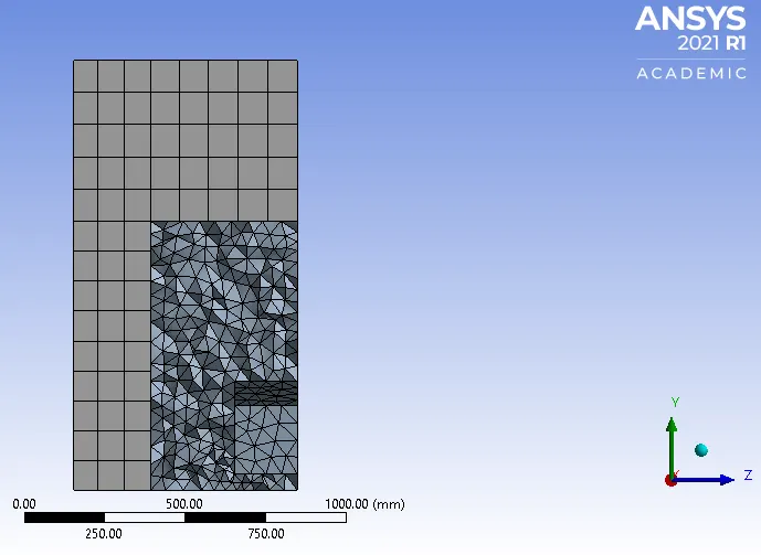
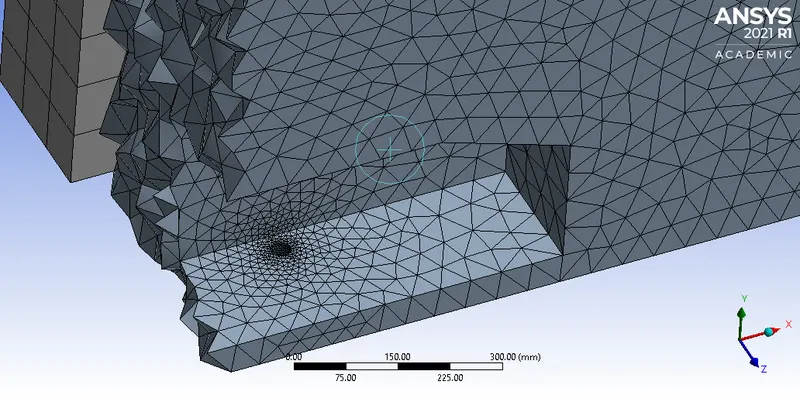
These huge mesh elements around the boundary has nodes away from the actual boundary and this might be a reason which could cause the calculations to deviate from the actual value.
So to create an inflation layer around the 'Ahmed body' would solve this issue.
These layers follow the boundary layer and creates accurate predictions.
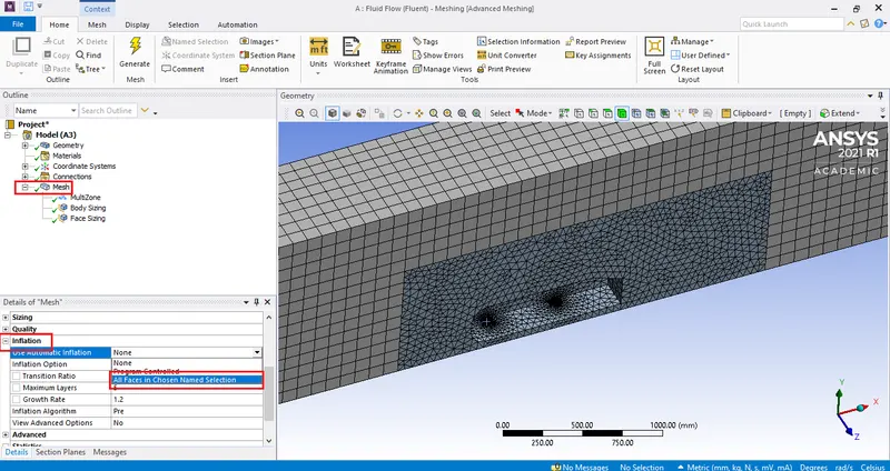
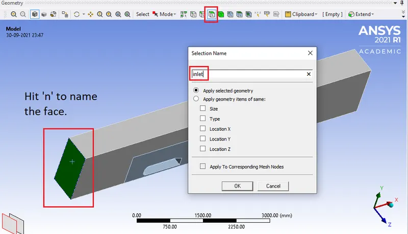
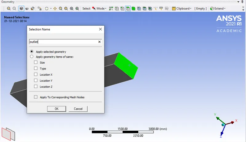
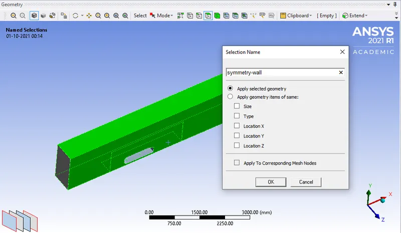
Now since the boundary hasn't been named. Naming has to be done before proceeding with creation of inflation layer.
To name the boundary follow the below procedure.
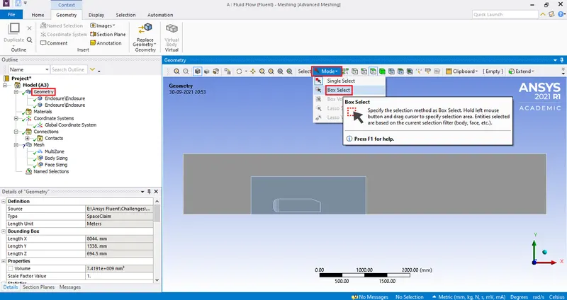
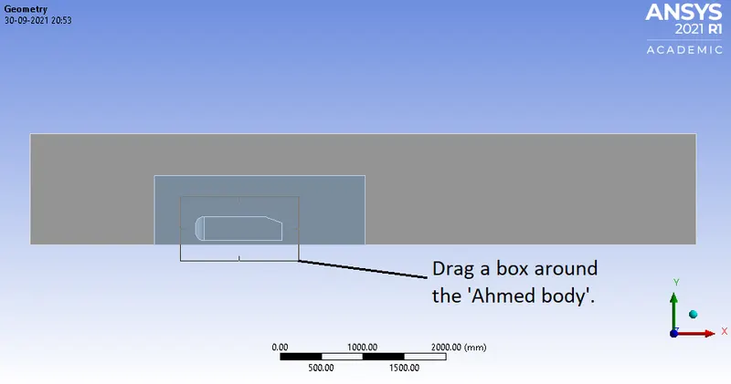
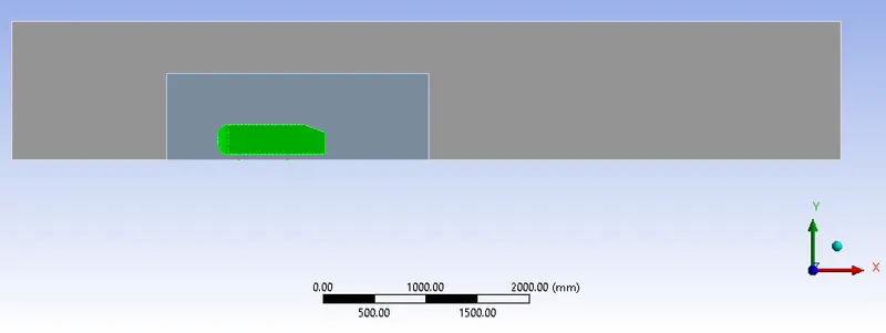
After the selection has been made hit 'n' to name the selection.
Name this boundary as 'car-wall'.
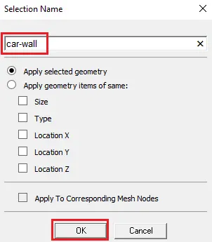
Now that the boundary has been named, the inflation layer has to be created.
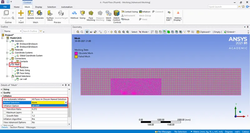
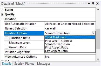
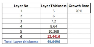
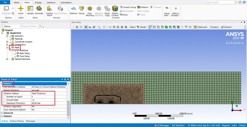
Specify this dimension in the details of mesh.
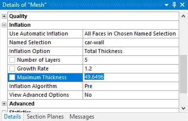
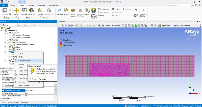
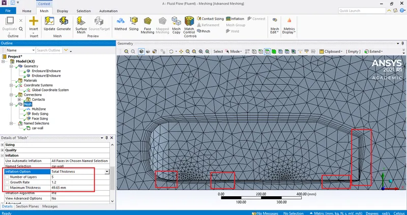
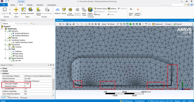
The irregularities in inflation layers are similar in both the 'first layer thickness' approach and also in the 'total layer thickness' approach.
So it really doesn't matter which inflation option we use.
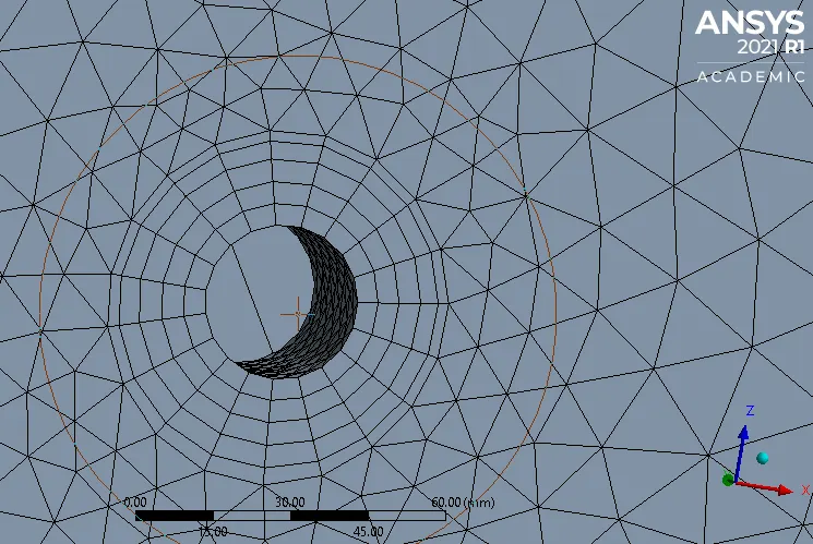
Effect of inflation layer on the bottom of the bluff body.
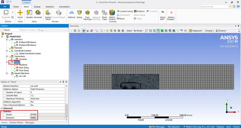
Close the meshing interface.
Open the setup.
Note:
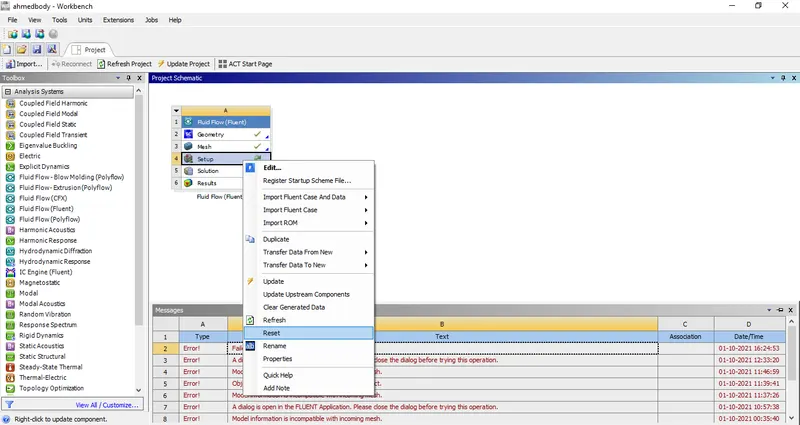
When new named selections are given hit reset before opening setup.
Setup:
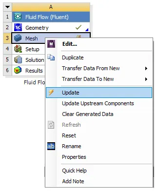
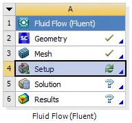
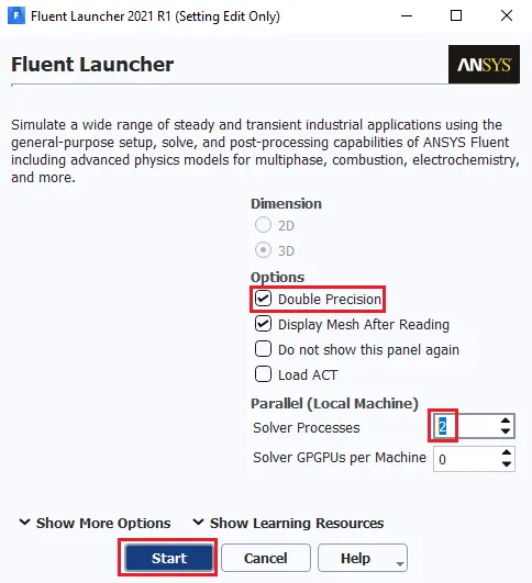
Start with checking the mesh.
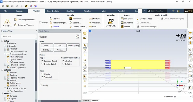
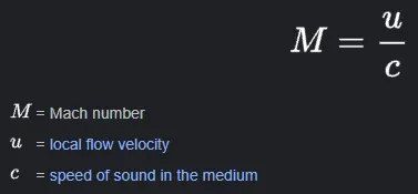
Since the velocity has been decided to be 25m/s and the speed of sound at sea level is 340.197m/s.
Then the mach number would be `(25(m/s))/(340.197(m/s))=0.07349`.
Since the mach number is lesser than 0.3, hence a pressure based solver must be used.
If the mach number is greater than 0.3 then the density based solver must be chosen.
For time accurate results a transient or unsteady simulation must be selected.
Perform check mesh to see if the mesh is ready to be used for simuation.
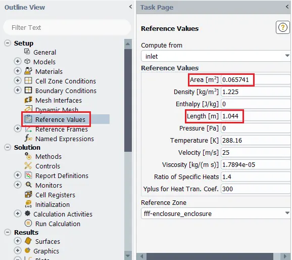
Projected area:
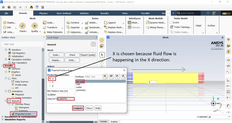
Characteristic length:
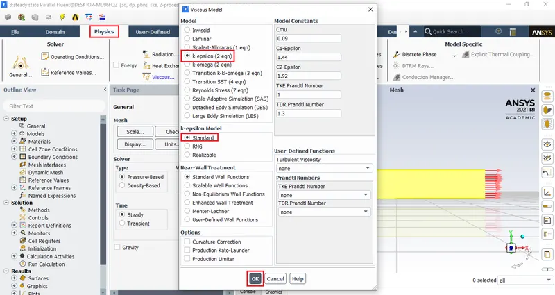
Since the focus here is to find the drag coeffecient of the 'Ahmed body' k-epsilon model can be chosen because this viscous model gives better results for large
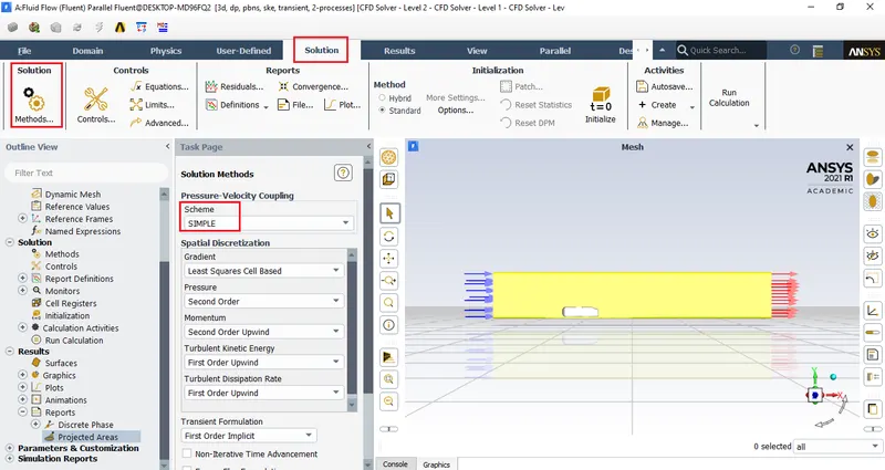
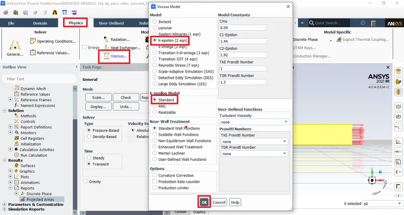

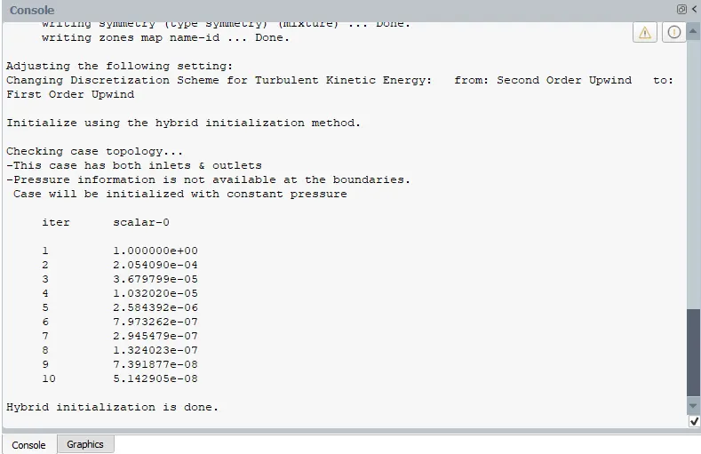
The idea is to solve for potential flow variables to get an estimate for the velocity components.
Here a value for pressure isn't possible but only the value for velocity is possible.
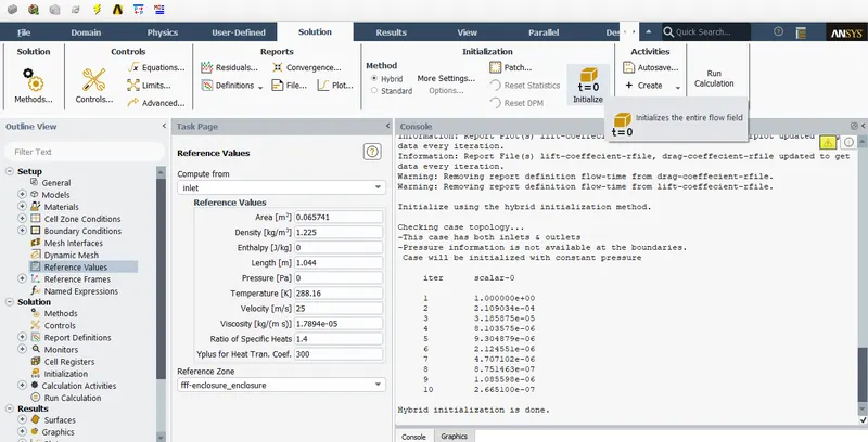
This provides a very good initial condition/starting point.
It's not an accurate approximation, it's a very good starting point when the flow path is really complex.
A PDE is obtained when you need to solve iteratively that's what happens when the solution is 'initialized'.
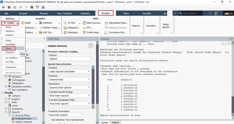
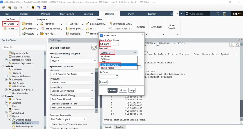
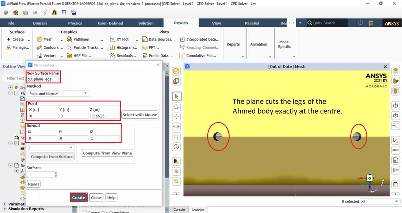
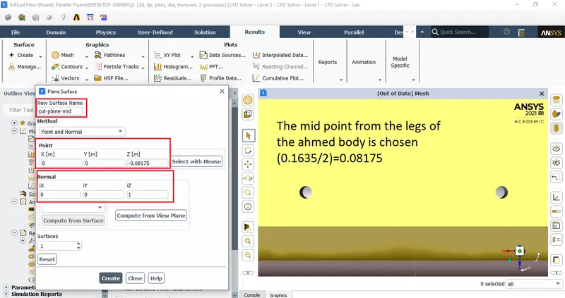
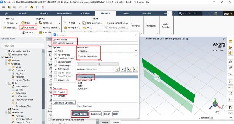
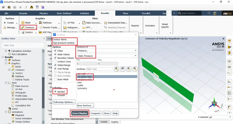
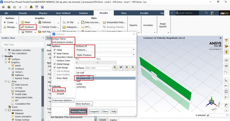
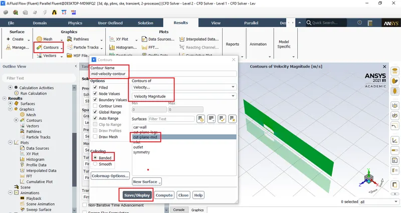
Hit create to generate a plane at this location.
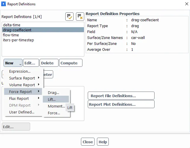
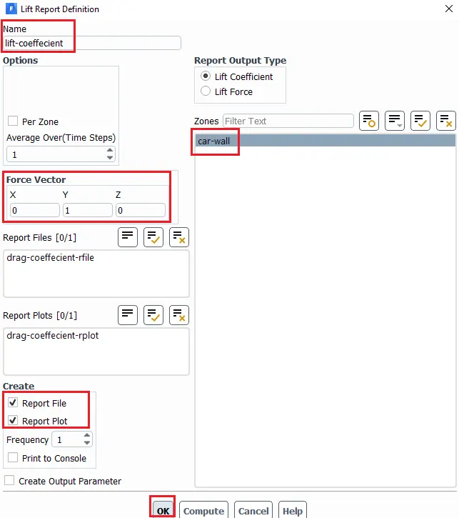
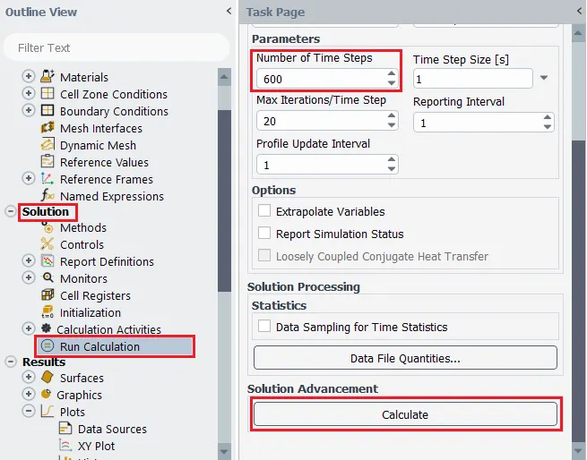
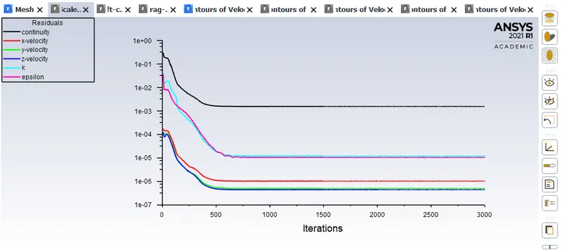
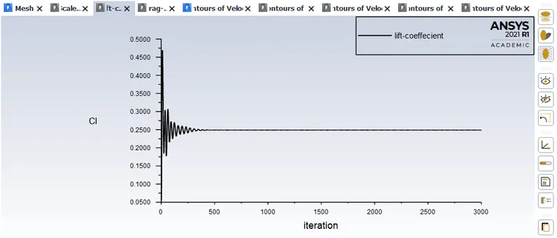
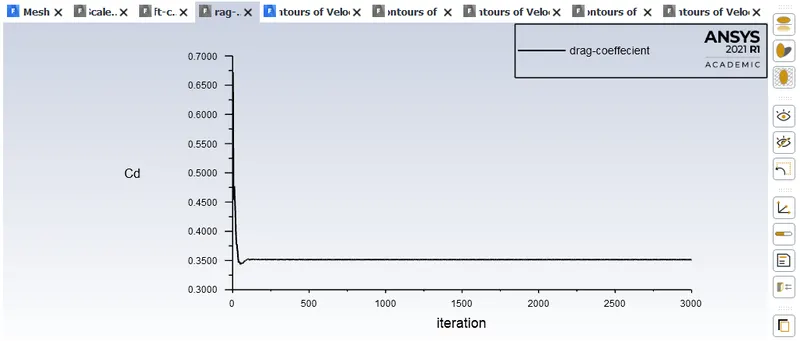
Results & plots for transient state:
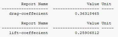
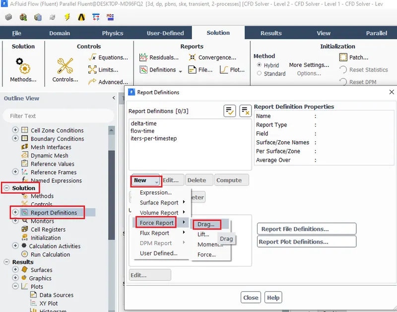
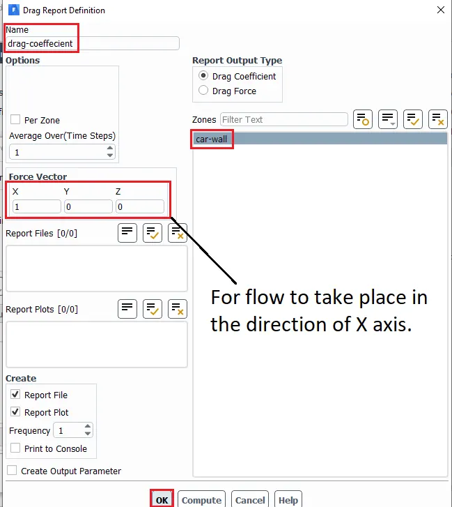
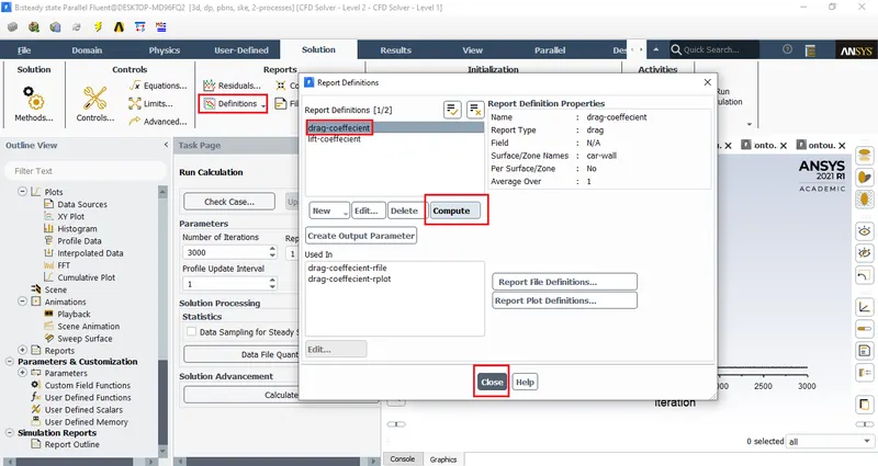
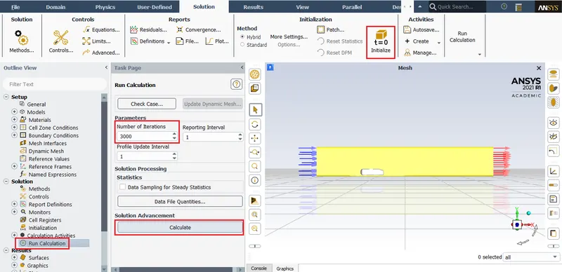
Solutions>Reports>Definition>Edit>Under 'Report definitions' :Select 'Lift or drag coeffecient>Compute.
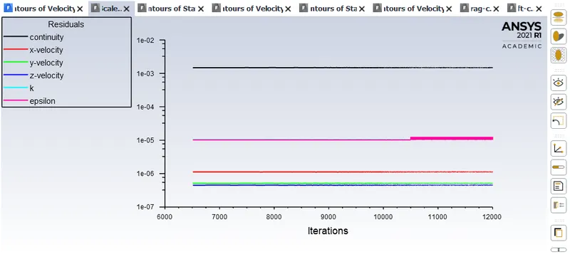
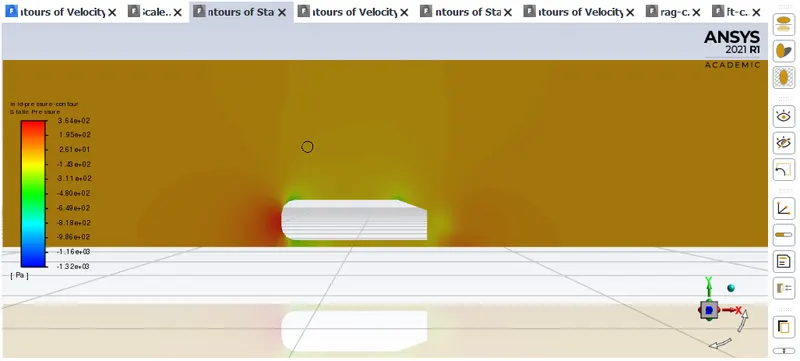
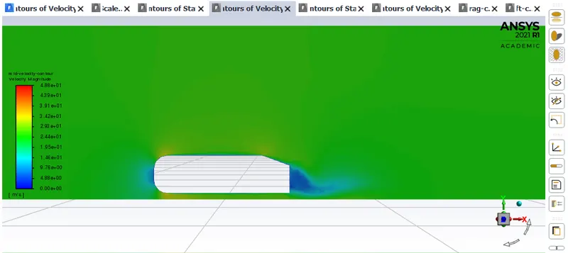
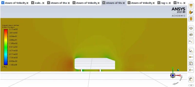
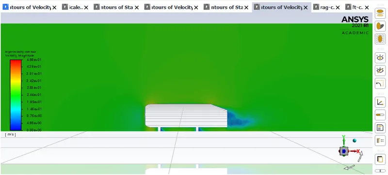
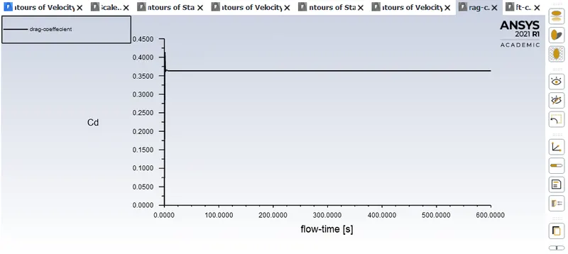
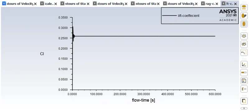
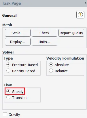
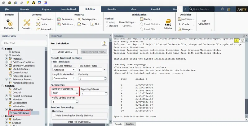
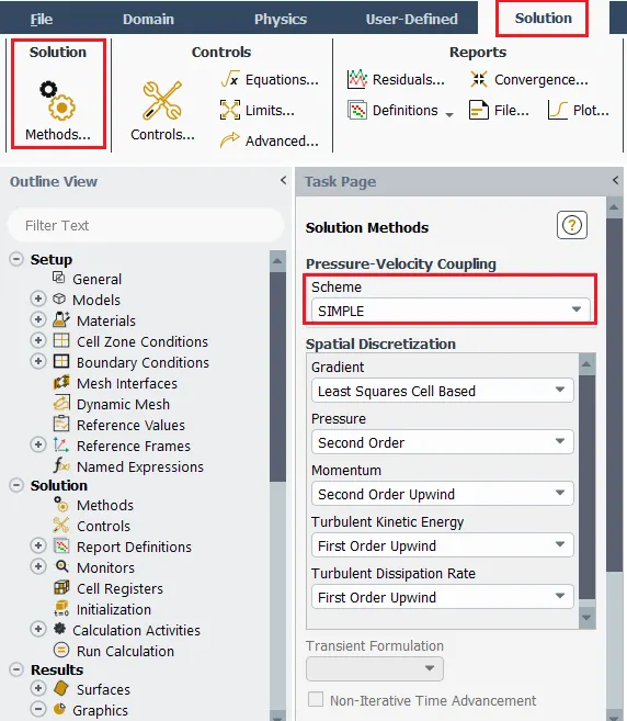
2) Steady state: The same procedure which was followed for the above case is followed for this case.
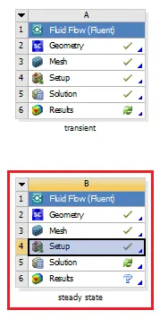

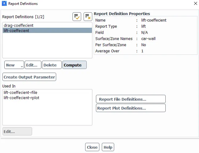
Results & plots for steady state:
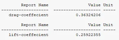
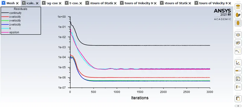
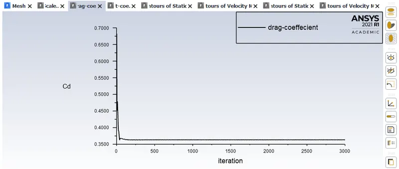
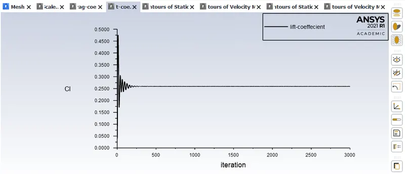
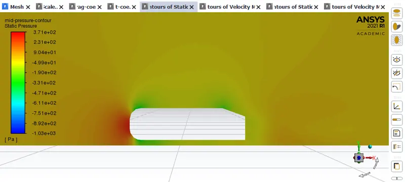
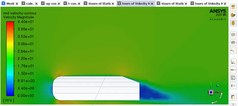
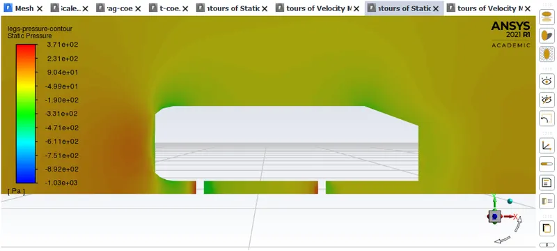
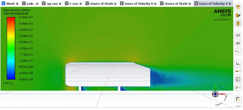
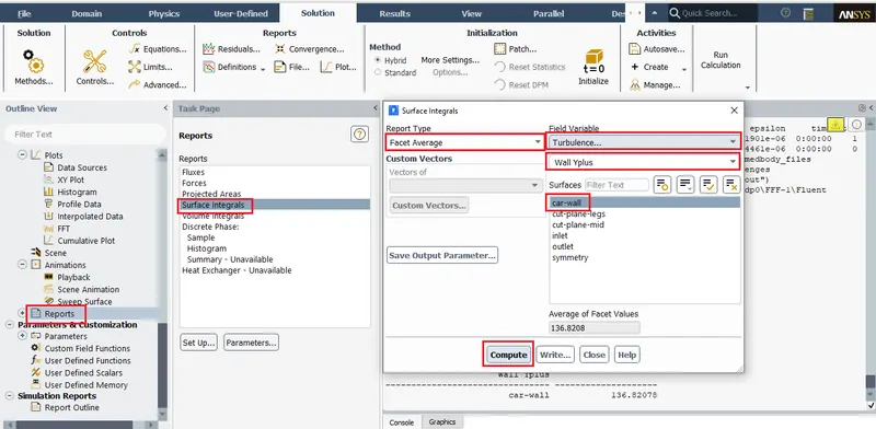
Results>Reports.

3) Realizable K-Epsilon model:
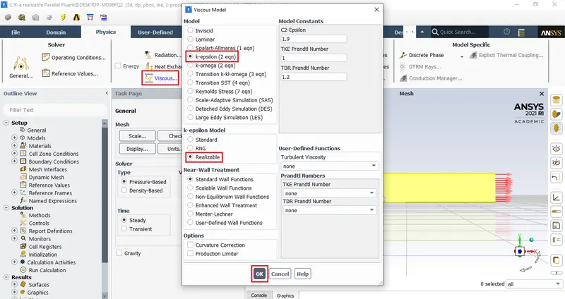
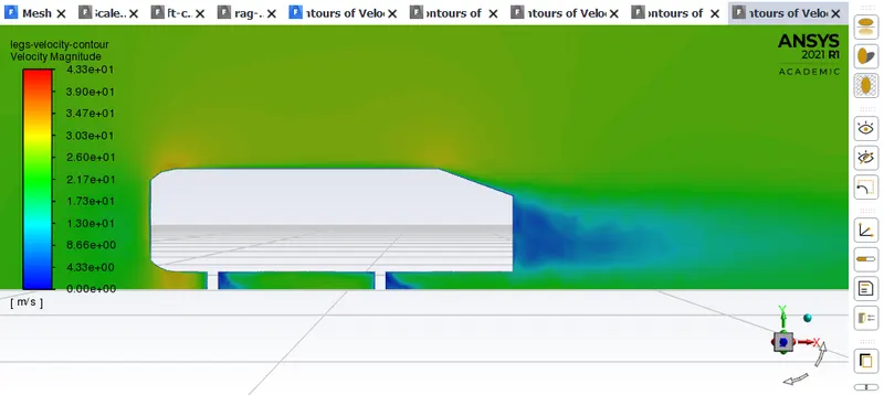
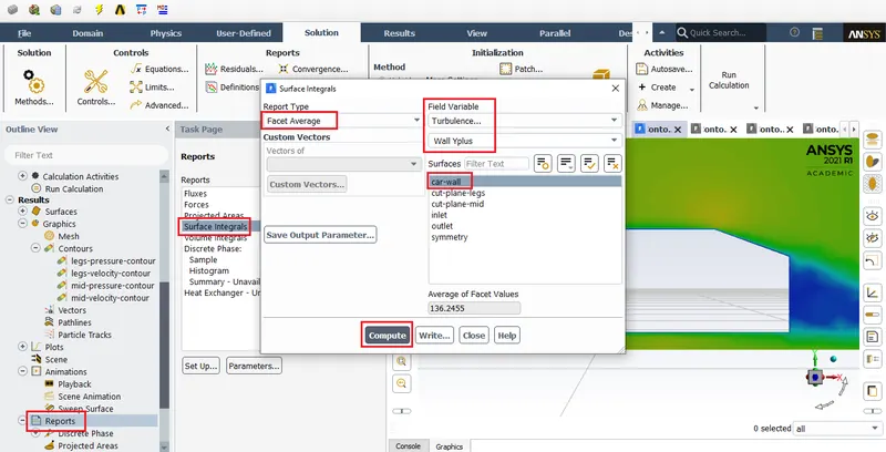
K-Omega SST:
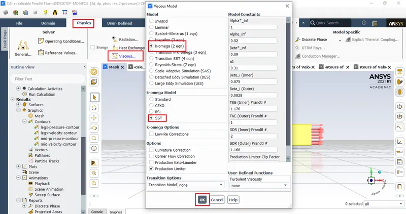
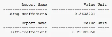
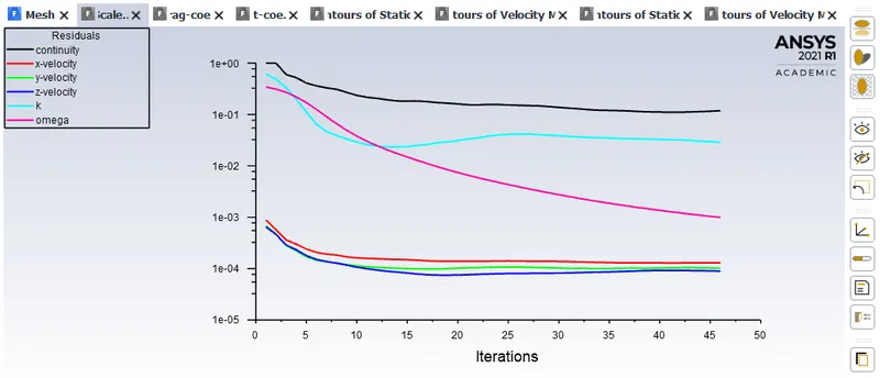
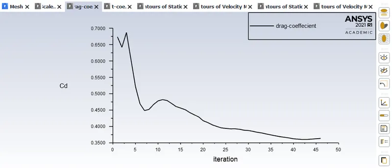
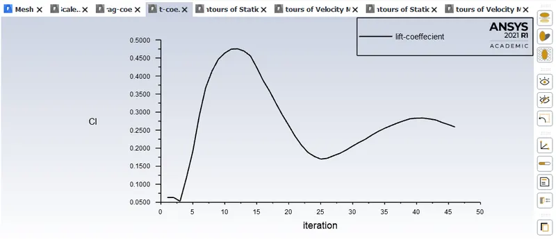
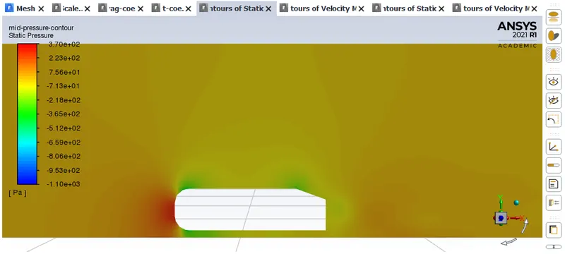
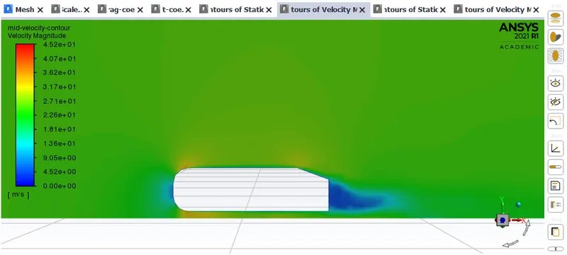
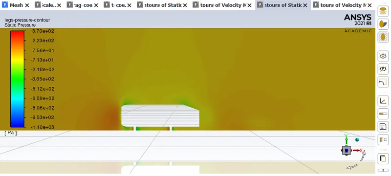
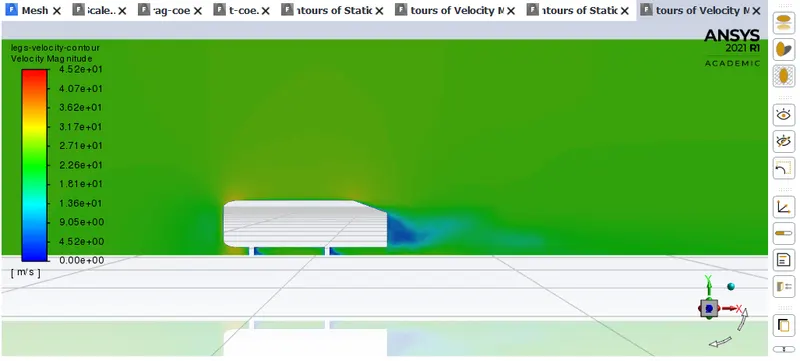
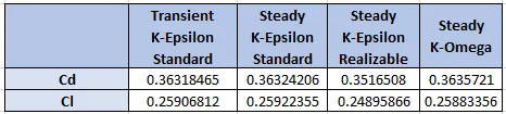
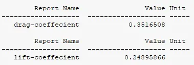
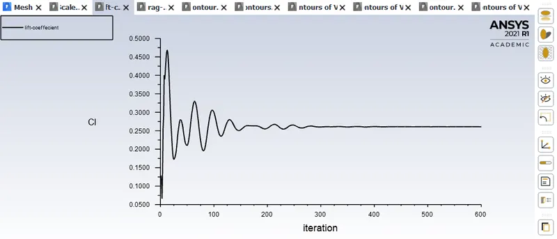
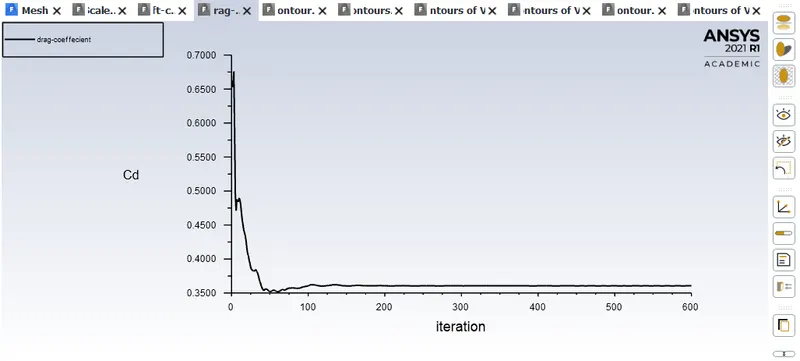
The coeffecient of drag value obtained from steady state K-Epslion(Realisable), is close to 0.33 which is the expected result. This value will be obtained after mesh refinement.
So the viscous model that will be used from further calculations will be Steady state K-Epsilon(Realisable).
Grid independency study:-
Mesh refinement:
Case 1:
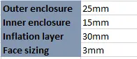
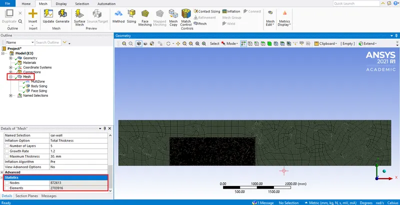
Element count exceeds ansys student license limit.
Case 2:
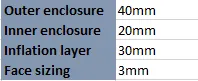
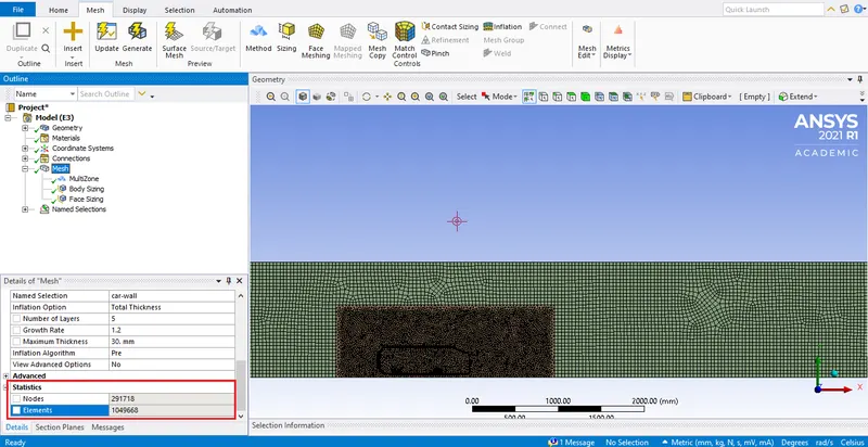
Element count exceeds ansys student license limit.
Case 3:
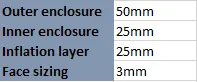
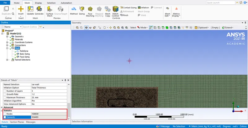
Element count exceeds ansys student license limit.
Case 4:
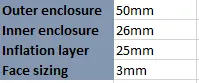
Inflation layer = total thickness.
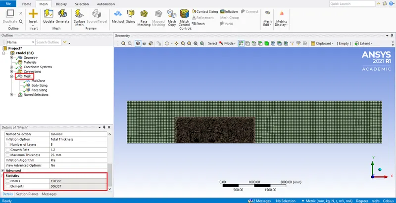
So at the above mentioned mesh dimensions, finest mesh within 512,000 limit is obtained.
For the ansys student license this is the finest possible mesh configuration.
So within this limit 2 random mesh configurations will be chosen over which the simulations will run.
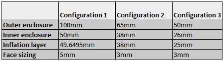
The above table shows the chosen mesh dimensions which whose results will be compared below.
1) Configuration 3:
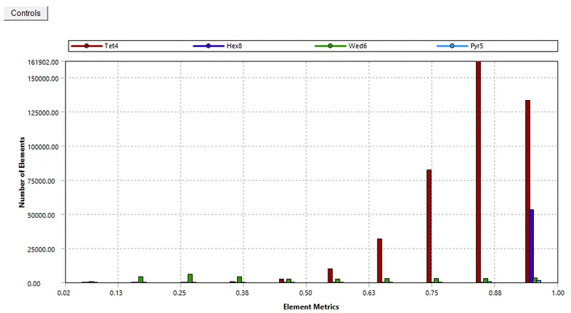
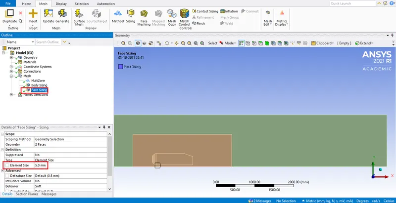
Mesh sizes:
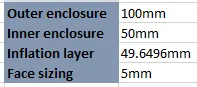
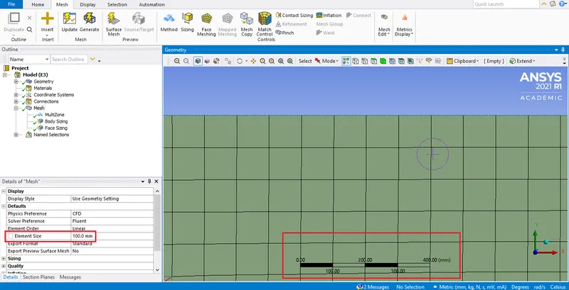
Setup:
Planes
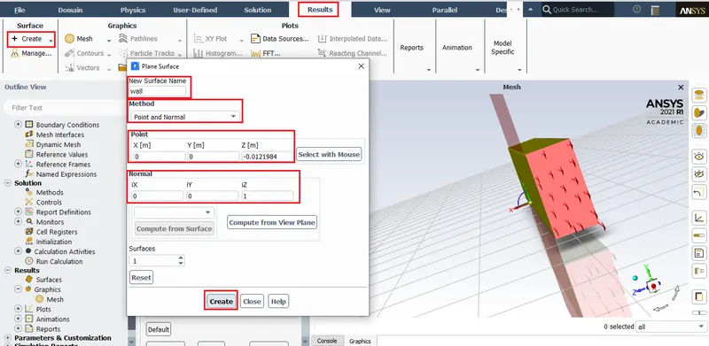
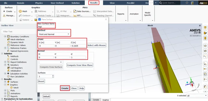
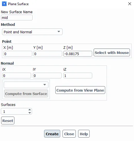
After creating the planes hit Initialize.
Results>Graphics>Contours.
Create a set of contours for each plane which shows both velocity and pressure variation.
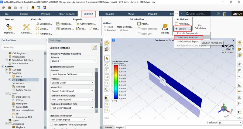
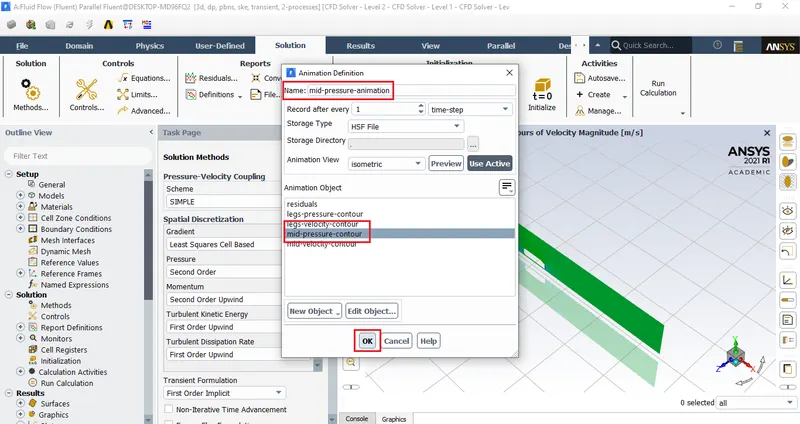
Solution>activities>create>Solution animation.

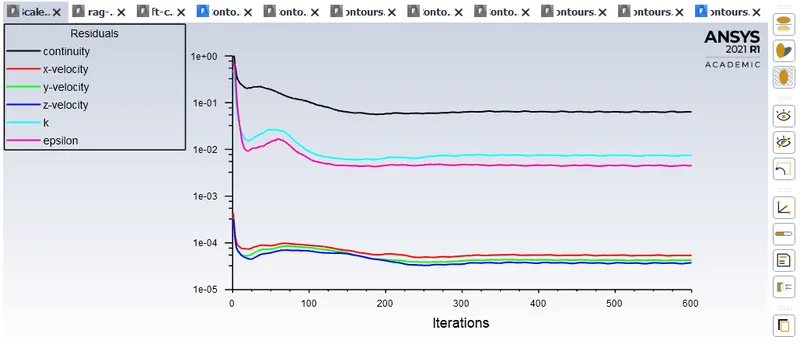
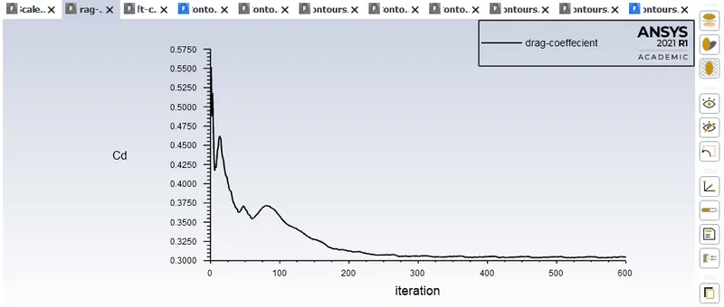
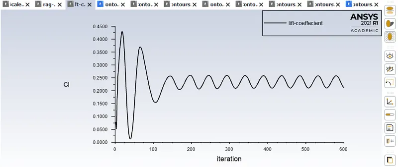
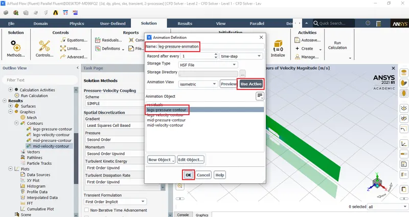
Pressure animation: leg plane
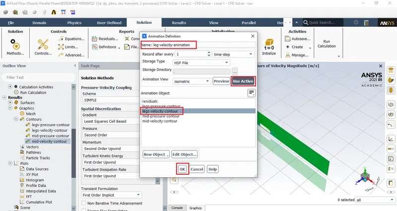
Velocity animation: leg plane
Pressure animation: mid plane
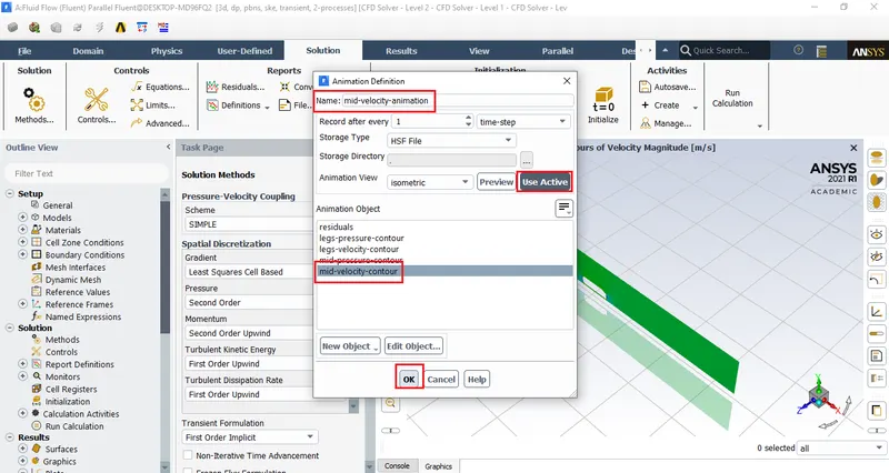
Velocity animation: mid plane
Pressure animation: Wall plane
Velocity animation: Wall plane
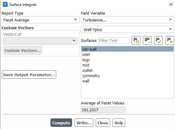
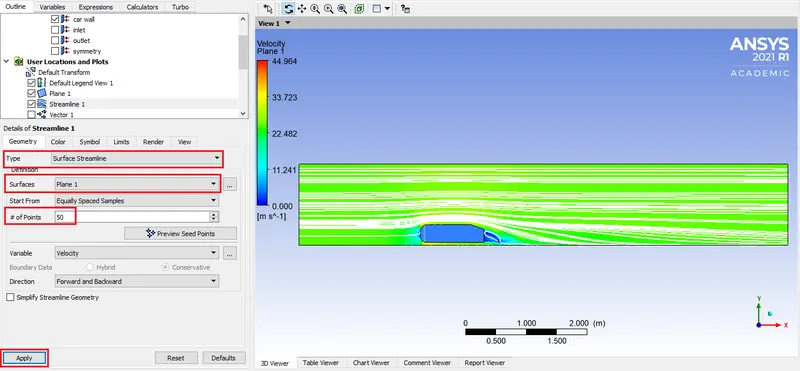
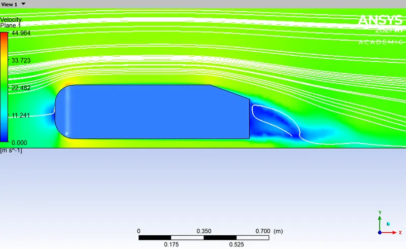
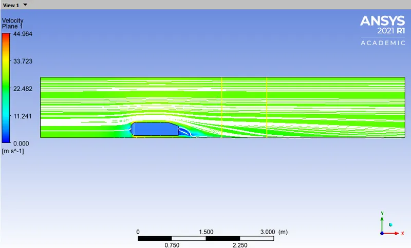
CFD Post:
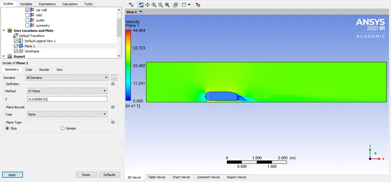
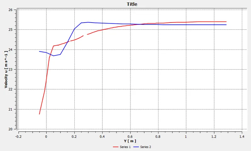
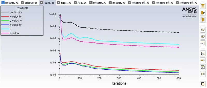
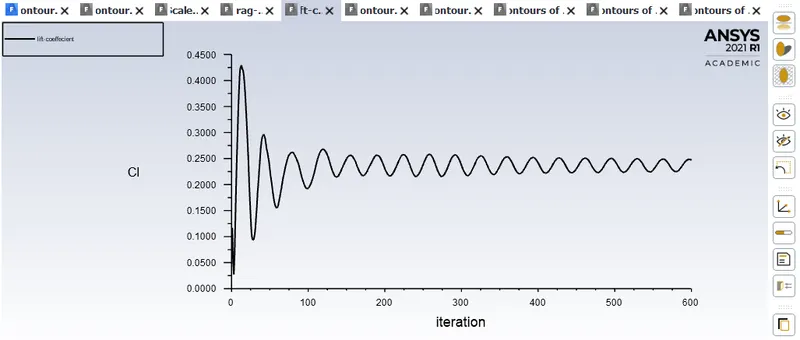
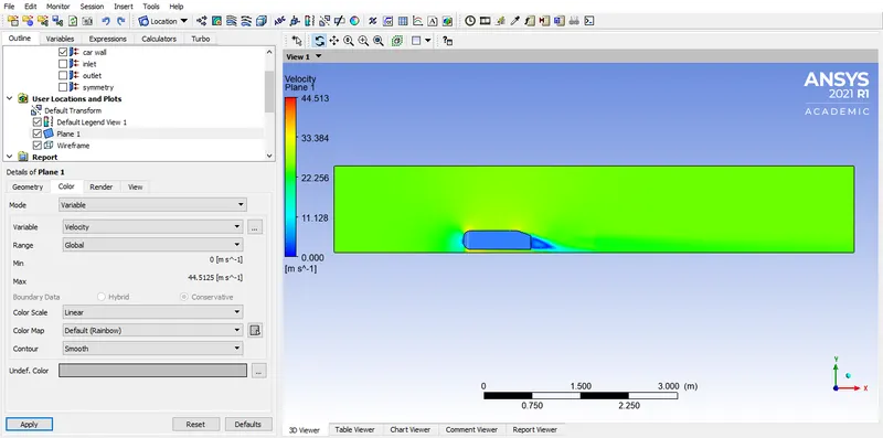
2) Configuration 2:
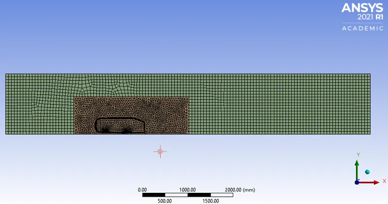
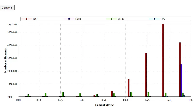
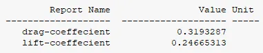
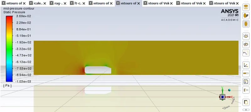
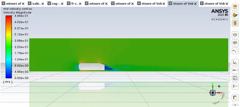
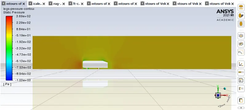
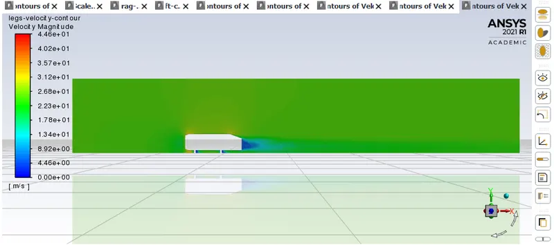
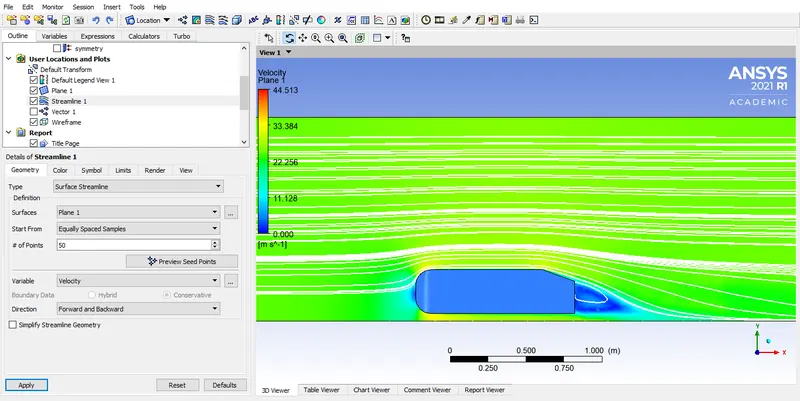
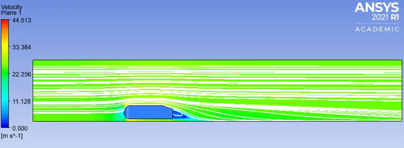
CFD Post:
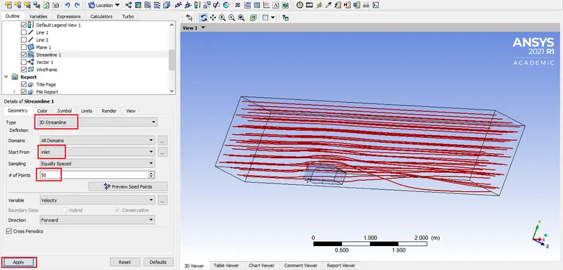
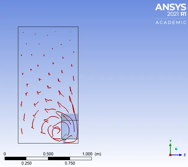
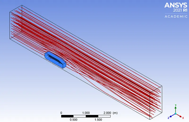
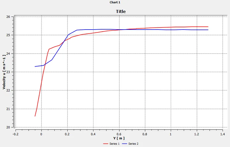
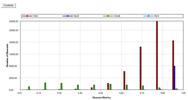
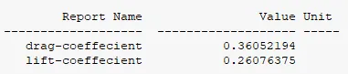
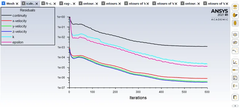
3) Configuration 1:
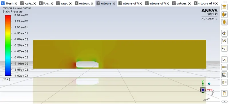
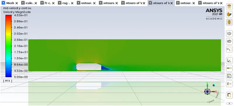
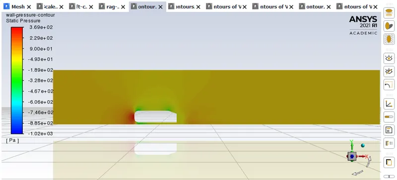
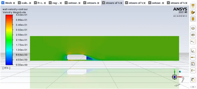
CFD Post:
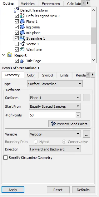
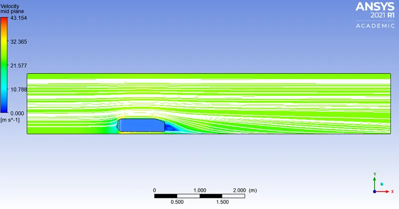
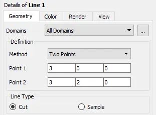
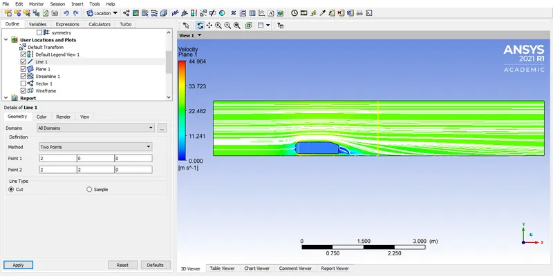
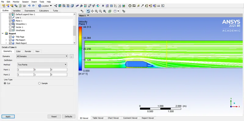
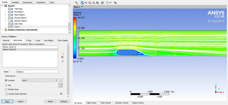
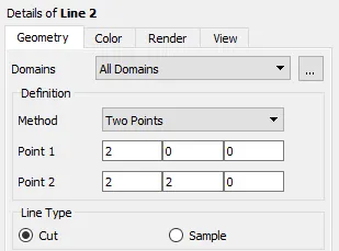
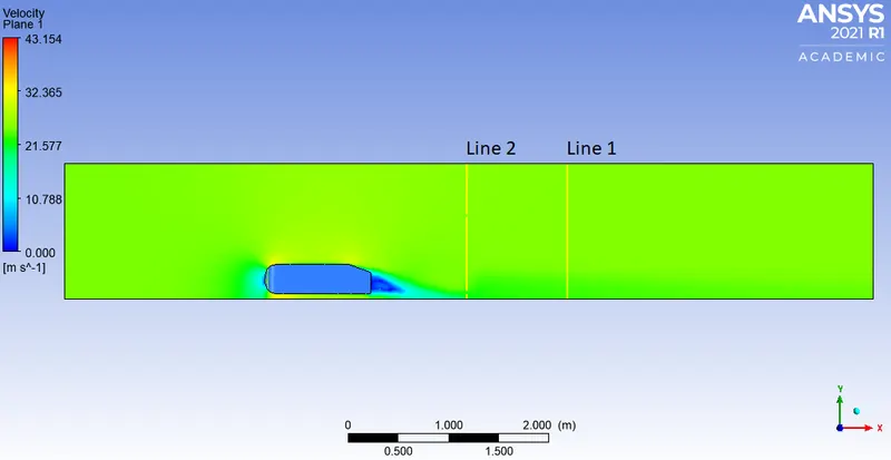
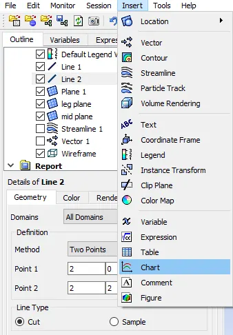
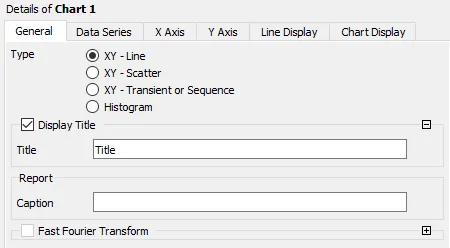
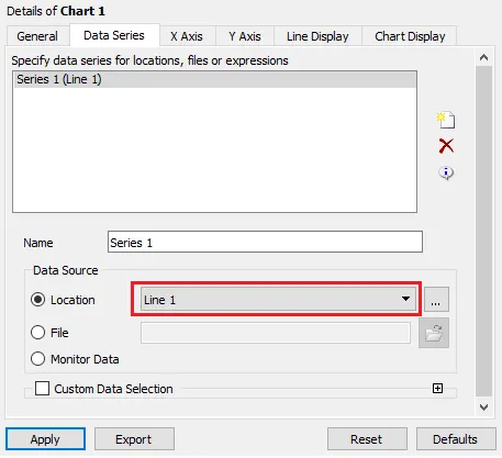
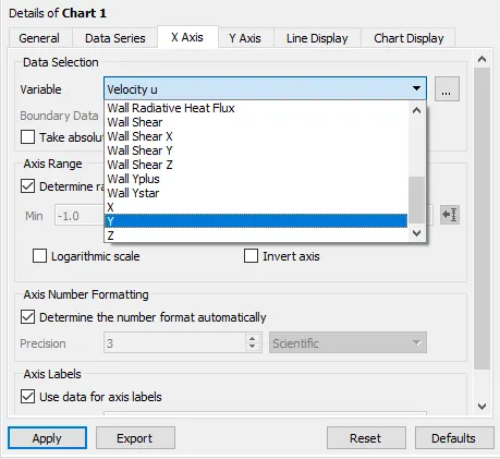
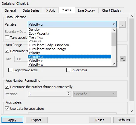
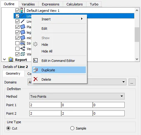
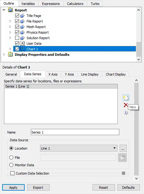
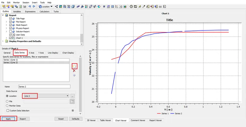
Insert>Location>Line>Ok
Reason for the negative pressure in the wake region:
The reason for negative pressure in wake region is due to formation of vortices. These vortices are localised zones of low pressure which decelerate a body in motion.
This is called the region of recirculation which is caused by viscosity of the fluid.
Point of seperation & its significance:
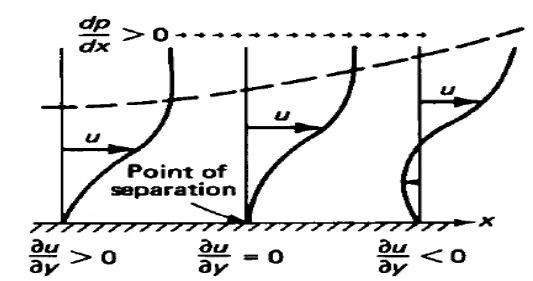
Separation of flow is said to occur when the direction of the flow velocity near the surface is opposed to the direction of the free stream velocity, which means (du/dy) ≤ 0. Such a situation arises when there is a negative pressure gradient near the wall (Refer figure below). An example is subsonic diffuser or rear portion of the car. In the direction of flow the pressure increases which causes decreases in velocity and creates condition for separation to occur.
It is important to note that, the skin-friction coefficient reaches the value zero. At this point the wall shear stress vanishes is called the separation point. Reverse flow takes place beyond point of separation. Due to reverse flow, irregular eddies are formed and lot of energy is dissipated. This region is called "Wake". The pressure distribution in the wake is quite different from that on the remaining boundary and this gives rise to an additional drag force on the body. Wake also leads to lateral vibration to the object which may be harmful. Also large amount of K.E. is lost.
In the turbulent boundary layer, some of the energy is dissipated in friction, slowing airflow velocity, resulting in a pressure increase. If the increase in pressure is gradual, the process of turbulent mixing will cause a transfer of energy from the fast moving eddies to slower ones in the turbulent boundary layer. If the rate of change in pressure is too great, for example in sharp corners, the mixing process will be too slow to push the slower air molecules moving. When this happens, the boundary layer flow stops following the contours of the surface, resulting in separation. Air particles downstream of the separation region will then move towards the lower pressure region in the reverse direction to the main flow, the separation region will reattach. In the region between separation and reattachment points, air flow is circulating and this is called the "separation bubble"
Results:
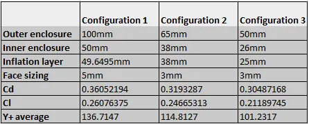
So the optimal mesh dimensions which produce meaningful results is found to be configuration 2.
Expected Cd value = 0.33 but the closest value for the same is found in configuration 2.
Error %:
Configuration 1: Error = `|(0.33-0.3604)/(0.33)*100|=9.212%`
Configuration 2: Error =`|(0.33-0.3192)/(0.33)*100|=3.2726%`
Configuration 3: Error =`|(0.33-0.3049)/(0.33)*100|=7.605%`
From above calculations it is safe to say that the configuration 2 produces best results.
References:
Ahmed body:
https://www.comsol.com/blogs/studying-the-airflow-over-a-car-using-an-ahmed-body/
https://drive.google.com/file/d/1la5_Od2O3YTy3Ez3EFFG9ExJJZYfnztd/view?usp=sharing
Split body tutorial:
https://www.youtube.com/watch?v=CRtPs0nt7jU
Y+ calculation:
https://skill-lync.com/knowledgebase/what-is-yplus
Y+ on ansys fluent:
https://www.youtube.com/watch?v=kecgPw-VmPU
Reynold's number:
https://www.grc.nasa.gov/www/k-12/airplane/reynolds.html
Fluid Mechanics: Fundamentals and Applications (3rd edition): Yunus Cengel & John M Cimbala(Third Edition)
https://drive.google.com/file/d/10AF8cJY4FoUIL3TwLNm6oucnx5J-Kkza/view?usp=sharing
K-epsilon: Standard vs Realizable.
https://www.researchgate.net/post/Difference-between-standard-and-realizable-k-epsilon-model
Wall Y+:
https://www.youtube.com/watch?v=kecgPw-VmPU
Flow seperation:
https://drive.google.com/file/d/1chHHrPnxUpHb4ymUK2LpsNJJjl1asyCG/view?usp=sharing
Other references:
https://drive.google.com/file/d/1wQgbmb-_2JeOPvtDufGq-1bAC5YqSkqh/view?usp=sharing
https://drive.google.com/file/d/11ncL19zb3JURlUJwvBIjKHyttPX7wlDV/view?usp=sharing
https://drive.google.com/file/d/1H6PFKC7OchqxW7PdkPiHODLyVQaEHwhl/view?usp=sharing
https://drive.google.com/file/d/1BdVE7tsYEyETmHT2TPYU0oQNJg2ymSYo/view?usp=sharing