Week 8 - Simulation of a backward facing step in OpenFOAM
BLOCKMESH :
The principle behind blockMesh is to decompose the domain geometry into a set of 1 or more three dimensional, hexahedral blocks. Edges of the blocks can be straight lines, arcs or splines. The mesh is ostensibly specified as a number of cells in each direction of the block, sufficient information for blockMesh to generate the mesh data.
Each block of the geometry is defined by 8 vertices, one at each corner of a hexahedron. The vertices are written in a list so that each vertex can be accessed using its label, remembering that OpenFOAM always uses the C++ convention that the first element of the list has label ‘0’.
Geometry :
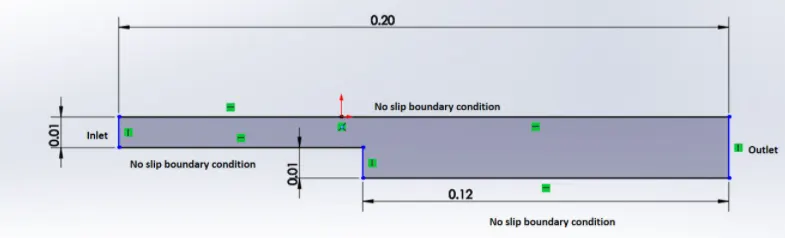
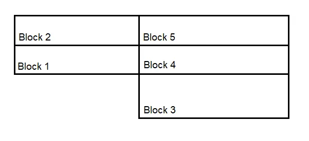
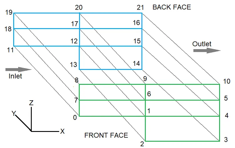
Commands in the terminal window :
- Firstly we must search for the tutorial that we will be using ,since this is an incompressible laminar viscous flow that we must simulate a solution for
Go to tutorials folder by typing 'tut' in the terminal window . - Since it is an incompressible flow open the 'incompressible' folder in 'openFOAM'
- Now again enter the 'icoFoam' folder and we can see 2 files here
- Open the 'cavity' folder and copy the 'cavity' folder to our run folder by typing 'cp -r cavity/ $FOAM_RUN/cav_test '
'cp' here is used to copy .
'-r' is used since we are copying a folder.
'cavity' is the folder that we intend to copy
'$FOAM_RUN' is the location at which we desire to paste the folder ,here we desire to copy the our tutorial in the folder 'run'.
'cav_test' is the new name that we give to the folder we are about to paste.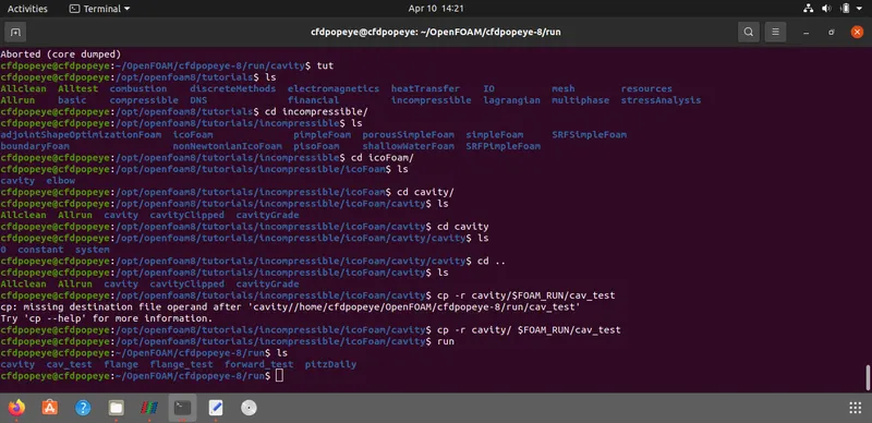
- Now we must find the solver that we can use to solve for this simulation we're desiring for .
In the terminal window :
Type 'sol' for accessing the solution folder
Select incompressible folder
Now enter the 'icoFoam' folder
To view what kind of equations are used in icoFoam solver use 'gedit icoFoam.C' to view the code that will get us our desired output.
icoFOAM solver :
icoFoam solves the incompressible laminar Navier-Stokes equations using the PISO algorithm. The code is inherently transient, requiring an initial condition (such as zero velocity) and boundary conditions. The icoFOAM code can take mesh non-orthogonality into account with successive non-orthogonality iterations. The number of PISO corrections and non-orthogonality corrections are controlled through user input.
icoFoam solver solves transient incompressible flows .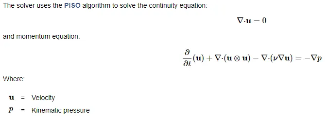
Mandatory input requirements :
- p: kinematic pressure [m2/s2]
- U: velocity [m/s]
This is why we find kinematic pressure in the code for pressure .
These links below explains the solver icoFoam in detail ,line by line
https://drive.google.com/file/d/1L7z9rm_7Tck4u_A3jbsW8fTDebvc-RRH/view?usp=sharing
https://drive.google.com/file/d/1zpWHFbVBeqImXDmJWc8KN3FyMFtZH3_q/view?usp=sharing
Note :
Below are a few things that need to be given a little more care to obtain a meaningful and desirable result .
1. CFL number : The CFL number must be lesser than 1 for us to generate a meaningful output ,if the CFL number exceeds values more than 1 the solution that we obtain might be faulty.
2. Inlet velocity : The inlet velocity that we specify should consider the length of the geometry and time taken for the simulation to run (present in the controlDict folder)
For this problem we choose inlet velocity 0.05 m/s & since the length of the geometry is 0.2m
The time taken for the simulation is 0.2/0.05 = 4 seconds .
To see the effects after the flow takes place ,we have given the simulation end time as 10 seconds .
3. Kinematic viscosity : We must choose a fluid for the simulation by choosing a kinematic viscosity .
Here ,we have taken kinametic viscosity of water which is 1e-6 at 20 degree celcius .
4. The front and back walls of the geometry must be of type empty because we do want to see what happens in between these walls .
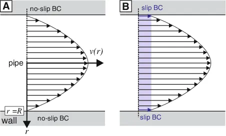
The other boundaries apart from the inlet and outlet boundaries must be set to a noslip condition this is because in fluid dynamics, the no-slip condition for viscous fluids assumes that at a solid boundary, the fluid will have zero velocity relative to the boundary. The fluid velocity at all fluid–solid boundaries is equal to that of the solid boundary.
Below is the of code which is common to both cases(case 1 & case 2) of our problem .
Velocity file :
/*--------------------------------*- C++ -*----------------------------------*
  =========                 |
  \      /  F ield         | OpenFOAM: The Open Source CFD Toolbox
   \    /   O peration     | Website:  https://openfoam.org
    \  /    A nd           | Version:  8
     \/     M anipulation  |
*---------------------------------------------------------------------------*/
FoamFile
{
    version     2.0;
    format      ascii;
    class       volVectorField;
    object      U;
}
// * * * * * * * * * * * * * * * * * * * * * * * * * * * * * * * * * * * * * //

dimensions      [0 1 -1 0 0 0 0];

internalField   uniform (0 0 0);

boundaryField
{
    inlet
    {
        type            fixedValue;
        value           uniform (0.05 0 0);
    }

    outlet
    {
        type            zeroGradient;
    }

    walls
    {
        type            empty;

    }

    noslipwalls
    {
    	type		 noSlip;
    }
}

// ************************************************************************* //
Here, from the above code we can say that the patch type inlet that we have specified in the blockMeshDict file is set to a fixed value of 0.05m/s
The outlet patch is set to zeroGradient means that the gradient of respective quantity is zero, meaning that the actual value is constant.
The front and back walls of the geometry is of type empty because at boundary we set boundary condition empty, flow is not solved in this direction .
The noSlip boundary condition is given to the top and bottom walls of the geometry & is an alternative to the zero fixedValue boundary condition for velocity. There is no difference between them .
Pressure file :
/*--------------------------------*- C++ -*----------------------------------*
  =========                 |
  \      /  F ield         | OpenFOAM: The Open Source CFD Toolbox
   \    /   O peration     | Website:  https://openfoam.org
    \  /    A nd           | Version:  8
     \/     M anipulation  |
*---------------------------------------------------------------------------*/
FoamFile
{
    version     2.0;
    format      ascii;
    class       volScalarField;
    object      p;
}
// * * * * * * * * * * * * * * * * * * * * * * * * * * * * * * * * * * * * * //

dimensions      [0 2 -2 0 0 0 0];

internalField   uniform 0;

boundaryField
{
    inlet
    {
        type            zeroGradient;
    }

    outlet
    {
        type 		 fixedValue;
	value 		 uniform 0;
    }

    walls
    {
        type            empty;
    }
    noslipwalls
    {
    	type            zeroGradient;
    }
}

// ************************************************************************* //
Here ,
1. The inlet kinematic pressure is set to zeroGradient
zeroGradient means that the gradient of respective quantity is zero, meaning that the actual value is constant. Ususally, pressure is taken to be zeroGradient at a inlet, because the pressure is assumed to be constant there .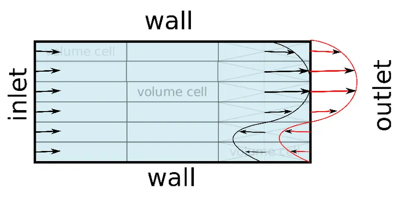
2. The uniformFixedValue boundary condition extends the fixedValue boundary condition .It sets the field to the uniform value as a function of time .It is applicable to all variables types (scalars, vectors, etc.)
3.The front and back walls are of type empty .
4.No slip walls are set to zeroGradient because we have assumed a no slip condition
Transport properties :
/*--------------------------------*- C++ -*----------------------------------*
  =========                 |
  \      /  F ield         | OpenFOAM: The Open Source CFD Toolbox
   \    /   O peration     | Website:  https://openfoam.org
    \  /    A nd           | Version:  8
     \/     M anipulation  |
*---------------------------------------------------------------------------*/
FoamFile
{
    version     2.0;
    format      ascii;
    class       dictionary;
    location    "constant";
    object      transportProperties;
}
// * * * * * * * * * * * * * * * * * * * * * * * * * * * * * * * * * * * * * //

nu              [0 2 -1 0 0 0 0] 1e-6; //dynamic viscosity of water


// ************************************************************************* //
Control dict file :
/*--------------------------------*- C++ -*----------------------------------*
  =========                 |
  \      /  F ield         | OpenFOAM: The Open Source CFD Toolbox
   \    /   O peration     | Website:  https://openfoam.org
    \  /    A nd           | Version:  8
     \/     M anipulation  |
*---------------------------------------------------------------------------*/
FoamFile
{
    version     2.0;
    format      ascii;
    class       dictionary;
    location    "system";
    object      controlDict;
}
// * * * * * * * * * * * * * * * * * * * * * * * * * * * * * * * * * * * * * //

application     icoFoam;

startFrom       startTime;

startTime       0;

stopAt          endTime;

endTime         10;

deltaT          0.005;

writeControl    timeStep;

writeInterval   20;

purgeWrite      0;

writeFormat     ascii;

writePrecision  6;

writeCompression off;

timeFormat      general;

timePrecision   6;

runTimeModifiable true;


// ************************************************************************* //
Case 1 - Simulate the flow without using any grading factor (i.e., GF = 1)
Mesh specification
- Number of cells along the x direction (longer dimension) = 200
- Number of cells along the z direction = 20
- Number of cells along the y direction = 1
BlockMeshDict file :
The naming of vertices ,blocks & boundaries need to be written keeping in mind the x,y,z coordinates in accordance with right hand thumb rule .
/*--------------------------------*- C++ -*----------------------------------*
  =========                 |
  \      /  F ield         | OpenFOAM: The Open Source CFD Toolbox
   \    /   O peration     | Website:  https://openfoam.org
    \  /    A nd           | Version:  8
     \/     M anipulation  |
*---------------------------------------------------------------------------*/
FoamFile
{
    version     2.0;
    format      ascii;
    class       dictionary;
    object      blockMeshDict;
}
// * * * * * * * * * * * * * * * * * * * * * * * * * * * * * * * * * * * * * //

convertToMeters 0.01;

vertices
(
    (0 0 0)     //v0
    (8 0 0)     //v1
    (8 0 -1)    //v2
    (20 0 -1)   //v3
    (20 0 0)    //v4
    (20 0 0.5)  //v5
    (8 0 0.5)   //v6
    (0 0 0.5)   //v7
    (0 0 1)     //v8
    (8 0 1)     //v9
    (20 0 1)    //v10
    (0 0.01 0)     //v11
    (8 0.01 0)     //v12
    (8 0.01 -1)    //v13
    (20 0.01 -1)   //v14
    (20 0.01 0)    //v15
    (20 0.01 0.5)  //v16
    (8 0.01 0.5)   //v17
    (0 0.01 0.5)   //v18
    (0 0.01 1)     //v19
    (8 0.01 1)     //v20
    (20 0.01 1)    //v21
);

blocks
(
    hex (0 1 12 11 7 6 17 18) (80 1 5) simpleGrading (1 1 1)      //B0
    hex (7 6 17 18 8 9 20 19) (80 1 5) simpleGrading (1 1 1)      //B1
    hex (2 3 14 13 1 4 15 12) (120 1 10) simpleGrading (1 1 1)    //B2
    hex (1 4 15 12 6 5 16 17) (120 1 5) simpleGrading (1 1 1)     //B3
    hex (6 5 16 17 9 10 21 20) (120 1 5) simpleGrading (1 1 1)    //B4
);

edges
(
);

boundary
(
    inlet
    {
        type patch;
        faces
        (

            (0 7 18 11)
            (7 8 19 18)
        );
    }
    outlet
    {
        type patch;
        faces
        (
            (21 10 5 16)
            (16 5 4 15)
            (15 4 3 14)
        );
    }
    walls
    {
        type empty;
        faces
        (
            //front
            (0 1 6 7)
            (7 6 9 8)
            (6 5 10 9)
            (1 4 5 6)
            (2 3 4 1)
            //back
            (11 18 17 12)
            (18 19 20 17)
            (17 20 21 16)
            (12 17 16 15)
            (13 12 15 14)
        );
    }
    noslipwalls
    {
    	type wall;
    	faces
    	(
    	     //top
            (8 9 20 19)
            (9 10 21 20)
            //bottom
            (0 11 12 1)
            (2 13 14 3)
            //bottomleftside
            (12 13 2 1)
    	);
    }
);

mergePatchPairs
(
);

// ************************************************************************* //
For simple grading 1
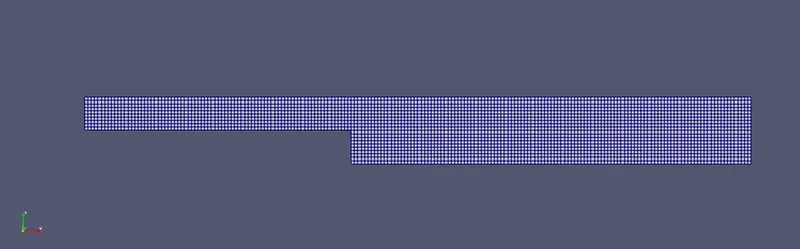
Case 1 mesh :
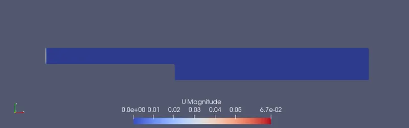
Case 1 at 0th time step for velocity :
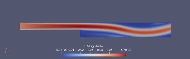
Case 2 at end time step for velocity :
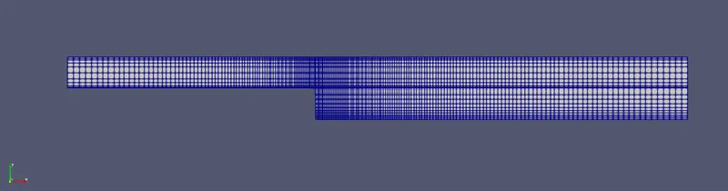
Case 2 - Simulate the flow with grading factor of 0.2 ,the cells should be finer near the walls (including the step wall).
Mesh specification
- Number of cells along the x direction (longer dimension) = 200
- Number of cells along the z direction = 20
- Number of cells along the y direction = 1
BlockMeshDict file :
The naming of vertices ,blocks & boundaries need to be written keeping in mind the x,y,z coordinates in accordance with right hand thumb rule .
/*--------------------------------*- C++ -*----------------------------------*
  =========                 |
  \      /  F ield         | OpenFOAM: The Open Source CFD Toolbox
   \    /   O peration     | Website:  https://openfoam.org
    \  /    A nd           | Version:  8
     \/     M anipulation  |
*---------------------------------------------------------------------------*/
FoamFile
{
    version     2.0;
    format      ascii;
    class       dictionary;
    object      blockMeshDict;
}
// * * * * * * * * * * * * * * * * * * * * * * * * * * * * * * * * * * * * * //

convertToMeters 0.01;

vertices
(
    (0 0 0)     //v0
    (8 0 0)     //v1
    (8 0 -1)    //v2
    (20 0 -1)   //v3
    (20 0 0)    //v4
    (20 0 0.5)  //v5
    (8 0 0.5)   //v6
    (0 0 0.5)   //v7
    (0 0 1)     //v8
    (8 0 1)     //v9
    (20 0 1)    //v10
    (0 0.01 0)     //v11
    (8 0.01 0)     //v12
    (8 0.01 -1)    //v13
    (20 0.01 -1)   //v14
    (20 0.01 0)    //v15
    (20 0.01 0.5)  //v16
    (8 0.01 0.5)   //v17
    (0 0.01 0.5)   //v18
    (0 0.01 1)     //v19
    (8 0.01 1)     //v20
    (20 0.01 1)    //v21
);

blocks
(
    hex (0 1 12 11 7 6 17 18) (80 1 5) simpleGrading (0.2 1 5)     //B0
    hex (7 6 17 18 8 9 20 19) (80 1 5) simpleGrading (0.2 1 0.2)   //B1
    hex (2 3 14 13 1 4 15 12) (120 1 10) simpleGrading (5 1 5)     //B2
    hex (1 4 15 12 6 5 16 17) (120 1 5) simpleGrading (5 1 5)      //B3
    hex (6 5 16 17 9 10 21 20) (120 1 5) simpleGrading (5 1 0.2)   //B4
);

edges
(
);

boundary
(
    inlet
    {
        type patch;
        faces
        (

            (0 7 18 11)
            (7 8 19 18)
        );
    }
    outlet
    {
        type patch;
        faces
        (
            (21 10 5 16)
            (16 5 4 15)
            (15 4 3 14)
        );
    }
    walls
    {
        type empty;
        faces
        (
            //front
            (0 1 6 7)
            (7 6 9 8)
            (6 5 10 9)
            (1 4 5 6)
            (2 3 4 1)
            //back
            (11 18 17 12)
            (18 19 20 17)
            (17 20 21 16)
            (12 17 16 15)
            (13 12 15 14)
        );
    }
    noslipwalls
    {
    	type wall;
    	faces
    	(
    	     //top
            (8 9 20 19)
            (9 10 21 20)
            //bottom
            (0 11 12 1)
            (2 13 14 3)
            //bottomleftside
            (12 13 2 1)
    	);
    }
);

mergePatchPairs
(
);

// ************************************************************************* //
For simple grading 0.2
Case 2 mesh :
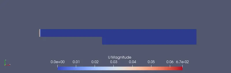
Case 2 at 0th time step for velocity :
Case 2 at end time step for velocity :
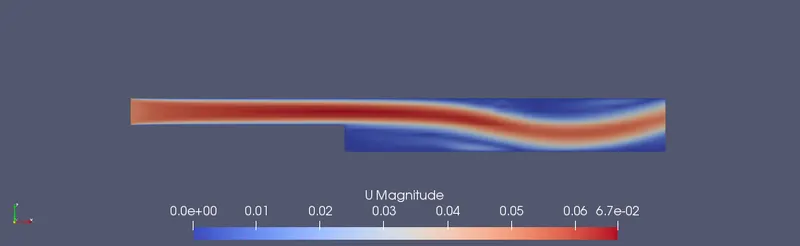
Vortex formation :
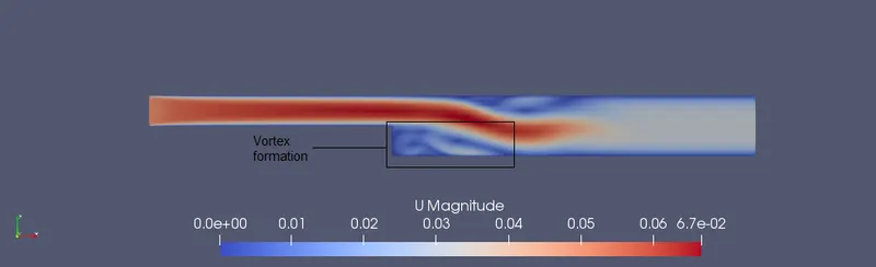
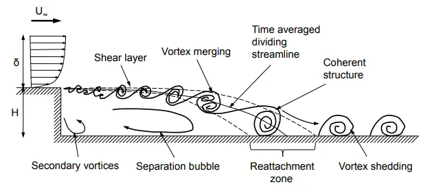
In a planar backward facing step geometry, the flow wake can be distinguished into three main regions namely, the shear layer region, separation bubble or recirculation zone and the reattachment zone. The general characteristics of a backward facing step flow begins with an upstream boundary layer separating at the step edge due to the adverse pressure gradient that develops into a thin shear layer. As the flow progresses downstream, the shear layer grows in size with the amalgamation of the turbulent structures contained within. This region where the shear layer develops and grows is referred to as the shear layer region. The turbulent structures in the shear layer entrain irrotational fluid from the non-turbulent region outside the shear layer. This flow entrainment causes the formation of a low velocity recirculation in the region, which is located between the shear layer and the adjacent wall. The recirculation zone is mainly comprised of a primary vortex in the center and a secondary vortex adjacent to the corner of the step Due to the favorable pressure gradient created by the fluid entrained, the shear layer eventually curves down towards the wall and impinges at a location known as the reattachment point. The horizontal distance between the step and the reattachment point is defined as the reattachment length. The reattachment length is unsteady due to the inherent oscillatory motion of the shear layer known as the flapping. As a result, the reattachment point spreads within a certain span along the streamwise distance, which is referred to as the reattachment zone. These three regions in a whole comprise the important features of a backward facing step flow that can be altered or controlled to achieve desirable outcome such as, enhanced mixing characteristics and reduced drag, noise and vibrations.
Results :
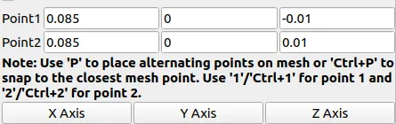
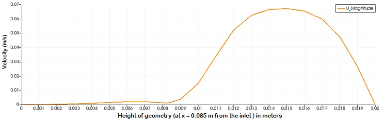
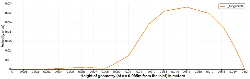
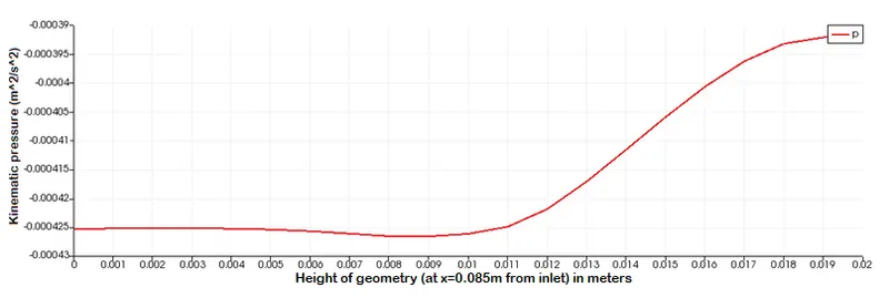
The values for dynamic pressure and velocity was plotted against the height of the geometry (z axis) at the coordinates mentioned below .
For case 1 : Simple grading 1
For case 2 : Simple grading 0.2
For case 1 : Simple grading 1
For case 2 : Simple grading 0.2
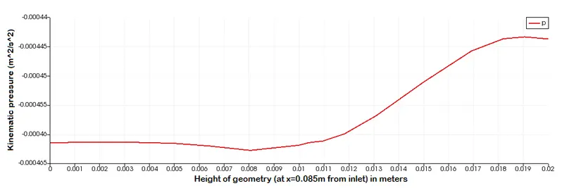
- From the above graph we can compare case 1 with case 2 ,the mesh is finer at the step in case 2 & the grading factor is 0.2 so the curves on the graph is finer in and around the 0.085m mark (this is done to view the flow seperation better than case 1) but produces rough edges elsewhere in the graph .
- Meanwhile ,the graph generated using simplegrading 1 (case 1) produces smooth curves throughout in both graphs of the same simple grading configuration
This is because the mesh is even throughout the geometry .
But the downside of doing this is that we are unable to capture the effect of flow seperation happening at the step in a detailed manner .