Week 9 - FVM Literature Review

What is Finite Volume Method(FVM) ?

The finite volume method discretises the governing equations by first dividing the physical space into a number of arbitrary polyhedral control volumes.

The finite-volume method is based on the fact that many physical laws are conservation laws—what goes into one cell on one side needs to leave the same cell on another side.

There are several possibilities of defining the shape and position of the control volume with respect to the grid. Two basic approaches can be distinguished:

• Cell-centred scheme (Fig. 1a) - here the flow quantities are stored at the centroids of the grid cells. Thus, the control volumes are identical to the grid cells.
• Cell-vertex scheme (Fig. 1b) - here the flow variables are stored at the grid points. The control volume can then either be the union of all cells sharing the grid point, or some volume centred around the grid point. In the former case we speak of overlapping control volumes, in the second case of dual control volumes.

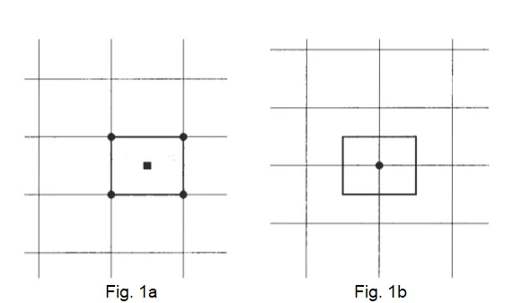
Fig. 1a : Control volume of cell-centred scheme .
Fig. 1b : Control volume of cell-vertex scheme (dual control volume).

FVM in brief :

• The properties are calculated for every cell instead of a node
• Based on the integral form of conservation laws and can handle discontinuities in solutions. In simple terms, what comes in, must go out.
• FVM approximates the value of the integral on the reference cell .
• Efficient in solving fluid flow problems.
• Like FEM, lot of established and theoretically proven subroutines are in place for FVM which can be directly implemented in the code.

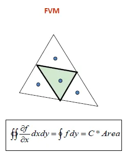
ADVANTAGES OF FVM :

The main advantage of the finite volume method is that the spatial discretisation is carried out directly in the physical space. Thus, there are no problems with any transformation between coordinate systems, like in the case of the finite difference method.
Compared to the finite differences, one further advantage of the finite volume method is that it is very flexible it can be rather easily implemented on structured as well as on unstructured grids. This renders the finite volume method particularly suitable for the treatment of flows in complex geometries.
Since the finite volume method is based on the direct discretisation of the conservation laws, mass, momentum and energy are also conserved by the numerical scheme. This leads to another important feature of the method, namely the ability to compute weak solutions of the governing equations correctly.

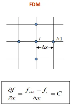
Finite Difference Method – FDM :

• Mostly for defined geometries which could be represented by structured grids
• This method is a subset of finite element method as it works mainly for structured spatial discretization. Which means, the problems solved by finite difference method could be solved using finite element method, but the converse is not necessarily true.
• One of the deviations in the case of FDM would come from approximating the higher order terms in Taylor’s series which is used to linearize the PDE. This is called as truncation error.
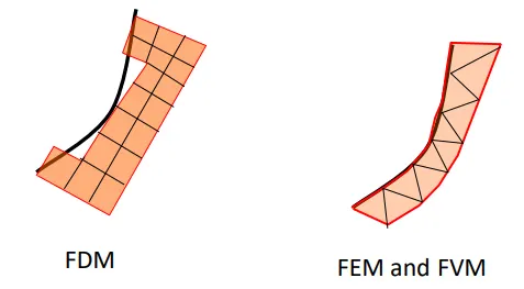
• Other important differentiating factor of FDM compared to FEM and FVM is that it is based on the differential form of governing equations. FEM and FVM are based on the integral form or weak formulation.

Comparison : FVM vs FDM vs FEM

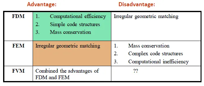
One disadvantage of FVM :
The local accuracy of the finite-volume method, such as close to a corner of interest, can be increased by refining the mesh around that corner, similar to the finite-element method. However, the functions that approximate the solution when using the finite-volume method cannot be easily made of higher order. This is a disadvantage of the finite-volume method compared to the finite-element and finite-difference methods.

Interpolation schemes :

Interpolation schemes are used to transform cell-centre quantities to face centres. The operation is used in many of the finite volume calculations for approximation of integrals other than CV nodes (CV centers), e.g. for the calculation of gradient, divergence, and laplacian terms.

1. Used to calculate
a)Convective & diffusive fluxes
b)Value of `phi` (where ,`phi` is a measurable quantity that is being approximated)
c)Gradient normal of `phi` to cell face at various locations on CV surface .
2. These have to be expressed in terms of nodal values by interpolation .
3. We shall show how the value of `phi` & it's normal derivative at the cell face 'e' can be approximated .

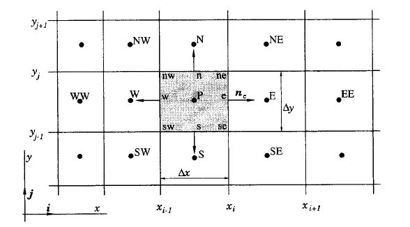
A typical CV and the notation used for a 2D cartesian grid

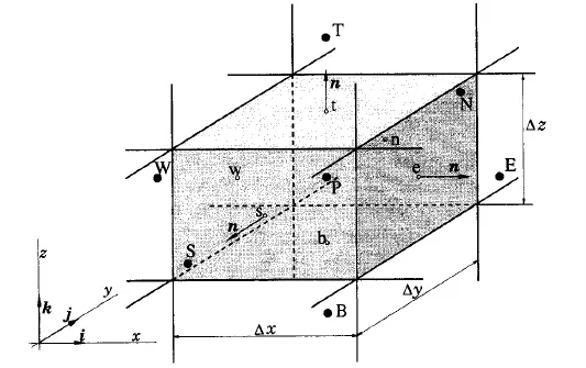
A typical CV and the notation used for a 3D cartesian grid

UDS (Upwind interpolation) :

Approximating `phi_e` by its value at the node upstream of 'e' is equivalent to using a backward or forward difference approximation for the first derivative (depending on the flow flow direction), hence the name 'Upwind differencing scheme(UDS)' for this approximation . In UDS ,`phi_e` is approximated as :
`phi_e = {(phi_P if (v.n)_e > 0 ;),(phi_E if (v.n)_e < 0 .):}`

This is the only approximation that unconditionally satisfies the boundedness criterion i.e. it will never yield oscillatory solutions. However ,it achieves this by numerically diffusive. This was shown in the preceding chapter and will be shown below .
Taylor's series expansion about P gives (for cartesian grid and `(v.n)_e > 0`) .
`phi_e = phi_P+(x_e-x_P).((delphi)/(delx))_P+(x_e-x_P)^2/2.((delphi)/(delx))_P+H`

where H denotes higher order terms .The UDS approximation retains only the first term on the right-hand side,so it is a first-order scheme. Its leading truncation error term is diffusive i.e. it resembles a diffusive flux :
`f_e^d = Gamma_e((delphi)/(delx))_e`

The coeffecient of numerical ,artificial ,or false diffusion (it goes by various uncomplimentary names) is `Gamma_e^(n um)=(rho*u)_e*(Deltax)/2` .This numerical diffusion is magnified in multidimensional problem if the flow is oblique to the grid ;the truncation error then produces diffusion in the direction normal to the flow as well as in the streamwise direction, a particularly serious type of error .
Peaks or rapid variations in the variables will be smeared out and since the rate of error reduction is only first order, very fine grids are required to obtain accurate solutions.

Linear Interpolation (CDS) :

Another straightforward approximation for the value at control volume face center is linear interpolation between the two nearest nodes. At location 'e' on a Cartesian grid we have

`phi_e=phi_Elambda_e+phi_P(1-lambda_e)`

where the linear interpolation factor `lambda_e` is defined as:

`lambda_e=(x_e-x_P)/(x_E-x_P)`

The above equation is a second order accurate as can be shown by using the taylor series expansion of `phi_E` about the point `x_P` to eliminate the first order derivative in Upwind interpolation scheme .

The result is :

`phi_e = phi_P+(x_e-x_P).((delphi)/(delx))_P+((x_e-x_P)(x_E-x_e))/2.((del^2phi)/(delx^2))_P+H`

The leading truncation error term is proportional to the square of the grid spacing on uniform or non uniform grids .

As with all approximations of order higher than one ,this scheme may produce oscillatory solutions .This is the simplest srcond-order scheme and is the one most widely used. It corresponds to the central-difference approximation of the first derivative in FD methods; hence the acronym CDS.
The assumption of a linear profile between the P & E nodes also offers the simplest approximation of the gradient ,which is needed for the evaluation of difusion fluxes:

`((delphi)/(delx))_e~~(phi_E-phi_P)/(x_E-x_P)`

By using taylor series expansion around `phi_e` one can show that truncation error of the above approximation is :

`in_r = ((x_e-x_P)^2-(x_E-x_e)^2)/(2(x_E-x_P))*((del^2phi)/(delx^2))_e-((x_e-x_P)^2-(x_E-x_e)^2)/(6(x_E-x_P))*((del^3phi)/(delx^3))_e+H`

When the location 'e' is midway between P & E (for example on a uniform grid), the approximation is of second order accuracy ,since the first term on the right hand side vanishes and the leading error term is then proportional to the product od `Deltax`and the grid expansion factor minus unity .In spite of the factor first-order accuracy ,the error reduction when the grid is refined is similar to that of a second-order approximation even on non-uniform grids.

Quadratic Upwind Interpolation (QUICK) :

Interpolation of order higher than third makes sense only if the integrals are approximated using higher-order formulae. If one uses Simpson's rule in 2D for surface integrals, one has to interpolate with polynomials of at least degree three, which leads to interpolation errors of fourth order. For example, by fitting a polynomial

`phi(x) =a_0_+a_1x+a_2x^2+a_3x^3`

through the values of `phi`at four nodes (two on either side of 'e' : W ,P ,E & EE), one can determine the four coeffecients `a_i` and find `phi_e` as a function of the nodal values. For a uniform Cartesian grid, the following expression is obtained :

`phi_e=(27phi_P+phi_E-3phi_W-3phi_(E E))/48`

The same polynomial can be used to determine the derivative; we need only to differentiate it once to obtain:

`((delphi)/(delx))_e=a_1+2a_2x+3a_3x^2`

which, on a uniform Cartesian grid, produces:

`((delphi)/(delx))_e=(27phi_E-27phi_P-phi_W-phi_(E E))/(24Deltax)`

The above approximation is sometimes called fourth-order CDS .Of course ,both polynomials of higher degree and /or multi-dimensional polynomials can be used. Cubic splines, which ensure continuity of the interpolation function and its first two derivatives across the solution domain, can also be used (at some increase in cost).

Once the values of the variable and its derivative are obtained at the cell face centers, one can interpolate on the cell faces to obtain values at the CV corners. This is not difficult to use with explicit methods but the fourth-order scheme based on Simpson's rule and polynomial interpolation produces too large a computational molecule for implicit treatment. One can avoid this complexity by using the deferred-correction approach .

Another approach is to use the techniques employed to derive compact schemes in FD methods.

Other Schemes :

The approach used above can be used to derive nearly all of them. We shall describe a few of them briefly.

One can approximate `phi_e` by linear extrapolation from two upstream nodes, leading to the so called linear upwind scheme (LUDS).
This scheme is of second order accuracy but, as it is more complex than CDS and can produce unbounded solutions, the latter is a better choice.

Another approach, is to extrapolate from the upwind side, but along a streamline rather than a grid line (skew upwind schemes).
First- and second-order schemes corresponding to the upwind and linear upwind schemes have been proposed.
They have better accuracy than schemes based on extrapolation along grid lines. However, these schemes are very complex (there are many possible directions of flow) and a lot of inter polation is required.
Since these schemes may produce oscillatory solutions when the grid is not sufficiently fine and are difficult to program, they have not found widespread use.

It is also possible to blend two or more different approximations, which switches between UDS and CDS, depending on the local value of the Peclet number.
Blending of lower and higher-order schemes can be done to avoid unphysical oscillations, especially for compressible flows with shocks.

TVD (total variation diminishing) schemes :

The class of TVD (total variation diminishing) schemes has been specially formulated to achieve oscillation-free solutions and has proved to be useful in CFD calculations.
In TVD schemes the tendency towards oscillation is counteracted by adding an artificial diffusion fragment or by adding a weighting towards upstream contribution.
TVD is a property used in the discretisation of equations governing time-dependent gas dynamics problems.
More recently, schemes with this property have also become popular in general-purpose CFD solvers. Fundamentals of the development of TVD methodology involves a fair amount of mathematical background.

The basic upwind differencing scheme is the most stable and unconditionally bounded scheme, but it introduces a high level of false diffusion due to its low order of accuracy (first-order). Higher-order schemes such as central differencing and QUICK can give spurious oscillations or ‘wiggles’ when the Peclet number is high. When such higher-order schemes are used to solve for turbulent quantities, e.g. turbulence energy and rate of dissipation, wiggles can give physically unrealistic negative values and instability.

Flux limiters :

Flux limiters are used in high resolution schemes – numerical schemes used to solve problems in science and engineering, particularly fluid dynamics, described by partial differential equations (PDE's). They are used in high resolution schemes, such as the MUSCL scheme, to avoid the spurious oscillations (wiggles) that would otherwise occur with high order spatial discretization schemes due to shocks, discontinuities or sharp changes in the solution domain. Use of flux limiters, together with an appropriate high resolution scheme, make the solutions total variation diminishing (TVD) .

Flux limiters are also referred to as slope limiters because they both have the same mathematical form, and both have the effect of limiting the solution gradient near shocks or discontinuities. In general, the term flux limiter is used when the limiter acts on system fluxes and slope limiter is used when the limiter acts on system states (like pressure, velocity etc.).

The main idea behind the construction of flux limiter schemes is to limit the spatial derivatives to realistic values – for scientific and engineering problems this usually means physically realisable and meaningful values. They are used in high resolution schemes for solving problems described by PDEs and only come into operation when sharp wave fronts are present. For smoothly changing waves, the flux limiters do not operate and the spatial derivatives can be represented by higher order approximations without introducing spurious oscillations. Consider the 1D semi-discrete scheme below,

`(du_i)/dt+1/(Deltax_i)*[F(u_(i+1/2))-F(u_(i-1/2))]=0`

where ,
`F(u_(i+1/2))` & `F(u_(i-1/2))` represent edge fluxes for the ith cell. If these edge fluxes can be represented by low and high resolution schemes, then a flux limiter can switch between these schemes depending upon the gradients close to the particular cell, as follows,

`F(u_(i+1/2))=(f^(low))_(i+1/2)-phi(r_i)*((f^(low))_(i+1/2)-(f^(high))_(i+1/2))`
`F(u_(i-1/2))=(f^(low))_(i-1/2)-phi(r_i)*((f^(low))_(i-1/2)-(f^(high))_(i-1/2))`

`here ,
`f^(low)`= low resolution flux
`f^(high)`= high resolution flux
and
r represents the ratio of successive gradients on the solution mesh .ie.,
`r_i=(u_i-u_(i-1))/(u_(i+1)-u_i`

The limiter function is constrained to be greater than or equal to zero ,i.e., `phi(r)>=0`

Therefore, when the limiter is equal to zero (sharp gradient, opposite slopes or zero gradient), the flux is represented by a low resolution scheme. Similarly, when the limiter is equal to 1 (smooth solution), it is represented by a high resolution scheme. The various limiters have differing switching characteristics and are selected according to the particular problem and solution scheme. No particular limiter has been found to work well for all problems, and a particular choice is usually made on a trial and error basis.

Example 4.1 : Page 118 - An introduction to computational fluid dynamics - H K Versteeg

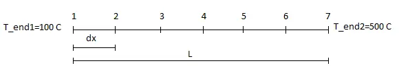
Consider the problem of source-free heat conduction in an insulated rod whose ends are maintained at constant temperatures of 100 C and 500 C respectively. The one-dimensional problem sketched in Figure is governed by `d/(dx)*(k*(dT)/(dx))=0`
Calculate the steady state temperature distribution in the rod. Thermal conductivity k equals 1000 W/m.K, cross-sectional area A is 10 × 10^(−3) m^2.

FVM :

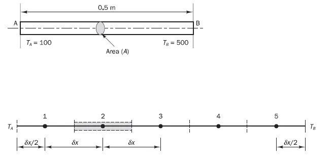
Iterative method used : Gauss siedel

Code : FVM

clear all 
close all
clc

ta=100;         % centigrade
tb=500;         % centigrade
a=10*10^(-3);   % m^2
l=0.5;          % m
k=1000;         % W/m.K 

format('long')  % for accuracy of upto 15 digits in calculation

n=5;

dx=l/n;

T=zeros(n);

tol=1e-5;
error=10;

for i = 1:n+2
    
if (i == 1)
x_x(i) = 0;
elseif (i == 2) 
    x_x(i) = dx/2;
elseif (i > 2) && (i < n+2) 
    x_x(i) = x_x(i-1)+dx;
elseif (i == n+2) 
    x_x(i) = l;
end

end

for i = 1:n

if (i == 1)
% for node 1
aw=0;
ae=k*a/dx;
sp=-(2*k*a)/(dx);
ap=aw+ae-sp;

% temprature 
T(i,i) = ap;
T(i,i+1) = -ae;

% source term 
su(i)=((2*k*a)/(dx))*ta;

elseif (i > 1) && (i < n)
% node 1 <= i <= n mid slab 
% for nodal points 2,3 & 4
aw=k*a/dx;
ae=k*a/dx;
ap=aw+ae;
% temprature 
T(i,i) = ap;
T(i,i+1) = -ae;
T(i,i-1) = -aw;

elseif (i == n)
% for node 5
ae=0;
aw=k*a/dx;
sp=-(2*k*a)/(dx);
ap=aw+ae-sp;

% temprature 
T(i,i) = ap;
T(i,i-1) = -aw;

% source term 
su(i)=((2*k*a)/(dx))*tb;
end

end

iter=0;
b=su';
x=[0;0;0;0;0];
while(error>tol)
    x_old=x;
    for i=1:size(T,1)
        sum=0;
        for j=1:i-1
            sum=sum+T(i,j)*x(j);
        end
        for j=i+1:size(T,1)
            sum=sum+T(i,j)*x_old(j);
        end
        x(i)=(1/T(i,i))*(b(i)-sum);
        x_new=x';
    end
    iter=iter+1;
%     y(iter,:)=x;
    error=abs(x_old-x);
end

% T_=su/T;
T_new=[ta x_new tb];

x_analytical=linspace(0,0.5,100);
t=800*x_analytical+100;

figure(1)
plot(x_analytical,t,'r','LineWidth',2)
hold on
grid on
plot(x_x,T_new,'xb','LineWidth',2)
xlabel('length of rod (m)')
ylabel('Temprature (C)')
legend('Exact solution','FVM solution')

• The first few lines of code declare quantities required for code .
• The first 'for loop' contains a few 'if statements' which produce 'x' values that will be useful to plot Temprature values .
• The second 'for loop' contains a few more 'if statements' which will be used to generate the elements of the temprature matrix and elements of the source term matrix .
  We use formulas generated from fvm concepts to populate the temprature matrix .
• The last part of the code is the gauss siedel iterative solver used to generate the temprature values
  For this we use a while loop that executes itself until (error>tol) value .
  Old values of x is stored before executing the code further.
  The first 'for loop' we encouner is used to calculate 5 temprature values that are unknown .
  The second 'for loop' is used to find the values of temprature using updated values of temprature from the neighbouring points .
  The thrid 'for loop' is used to generate values of elements of temprature matrix using old values of temprature because the new values haven't been calculated .
  We update the temprature values to find out the error which is very important to fullfil the error ,tolerance criteria .
• The we use the formula(T=800x+100) in the textbook to find the exact solution .
• We plot the exact solution and numerical solution to compare values from both methds to verify if the values we obtaines numerically are fair enough .

Output :
FVM numerical solution vs Exact solution

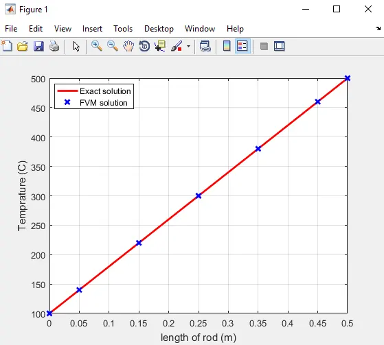
Here we can see clearly that the numerical solution matches with the exact solution .

FDM :

Code : FDM

clear all
close all
clc

n=6;
l=0.5;
dx=l/n;

T_end1=100;
T_end2=500;
T=zeros(5,5);
b=zeros(5,1);

format('long')  % for accuracy of upto 15 digits in calculation

for i = 1:n+1
    
if (i == 1)
x_x(i) = 0;
elseif (i > 1) && (i < n+2) 
    x_x(i) = dx+x_x(i-1);
elseif (i == n+1) 
    x_x(i) = l;
end

end

for i = 2:n
    
if (i == 2)
        b(i-1)=100;
        T(i-1,i-1)=2;
        T(i-1,i)=-1;

elseif (i > 2) && (i < n) 
        b(i)=0;
        T(i-1,i-2)=1;
        T(i-1,i-1)=-2;
        T(i-1,i)=1;
elseif (i == n)
     b(i-1)=500;
     T(i-1,i-1)=2;
     T(i-1,i-2)=-1;
end

end


iter=0;
x=[0;0;0;0;0];

tol=1e-5;
error=10;

while(error>tol)
    x_old=x;
    for i=1:size(T,1)
        sum=0;
        for j=1:i-1
            sum=sum+T(i,j)*x(j);
        end
        for j=i+1:size(T,1)
            sum=sum+T(i,j)*x_old(j);
        end
        x(i)=(1/T(i,i))*(b(i)-sum);
        x_new=x';
    end
    iter=iter+1;
%     y(iter,:)=x;
    error=abs(x_old-x);
end

% T_=su/T;

T_new=[T_end1 x_new T_end2];

x_analytical=linspace(0,0.5,100);
t=800*x_analytical+100;

figure(1)
plot(x_analytical,t,'r','LineWidth',2)
hold on
grid on
plot(x_x,T_new,'xb','LineWidth',2)
xlabel('length of rod (m)')
ylabel('Temprature (C)')
legend('Exact solution','FDM solution')

• The first few lines of code declare quantities required for code .
• The first 'for loop' contains a few 'if statements' which produce 'x' values that will be useful to plot Temprature values .
• The second 'for loop' contains a few more 'if statements' which will be used to generate the elements of the temprature matrix and elements of the source term matrix .
• The last part of the code is the gauss siedel iterative solver used to generate the temprature values
  For this we use a while loop that executes itself until (error>tol) value .
  Old values of x is stored before executing the code further.
  The first 'for loop' we encouner is used to calculate 5 temprature values that are unknown .
  The second 'for loop' is used to find the values of temprature using updated values of temprature from the neighbouring points .
  The thrid 'for loop' is used to generate values of elements of temprature matrix using old values of temprature because the new values haven't been calculated .
  We update the temprature values to find out the error which is very important to fullfil the error ,tolerance criteria .
• The we use the formula(T=800x+100) in the textbook to find the exact solution .
• We plot the exact solution and numerical solution to compare values from both methds to verify if the values we obtaines numerically are fair enough .

Output :
FDM numerical solution vs Exact solution

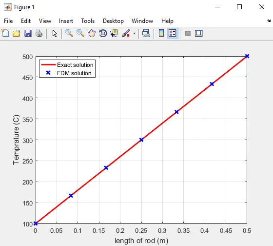
Here we can see clearly that the numerical solution matches with the exact solution .