Week 4 - CHT Analysis on Exhaust port

Introduction:

The Conjugate Heat Transfer (CHT) analysis type allows for the simulation of heat transfer between solid and fluid domains by exchanging thermal energy at the interfaces between them. Typical applications of this analysis type exist as, but are not limited to, the simulation of heat exchangers, cooling of electronic equipment, and general-purpose cooling and heating systems.

Internal Combustion Engines

The internal combustion engine industry is moving toward simulating the entire system rather than independent components. The accuracy of the predicted combustion in the cylinder is dependent on the temperature boundary conditions in the cylinder. By considering heat transfer in the metal components (e.g., the cylinder head, liner, piston, etc.), the cylinder wall no longer has a user-specified temperature, but instead has temperatures predicted as part of the complete-system simulation. This makes the overall simulation results more predictive by reducing the dependence on assumed boundary conditions.

Electromobility

Effective cooling strategies are critical for various components of emobility systems. Electric motors have high power densities and thus generate a significant amount of heat. If a motor is not properly cooled, high temperatures in the motor can cause the demagnetization of the permanent magnets and the breakdown of the winding insulation.
Types of cooling: Air cooling, water jacket cooling, and oil spray cooling.

For lithium-ion battery packs, CHT simulations are necessary for conducting cooling analyses under normal operating conditions and for predicting thermal runaway. Thermal runaway occurs when a cell reaches a temperature that triggers a cascade of exothermic reactions, causing the temperature to continue to increase. If a runaway cell will cause adjacent cells to initiate thermal runaway, which can be catastrophic to a battery pack.

Aftertreatment

Predicting and mitigating urea deposit formation is a key challenge in Urea/SCR aftertreatment systems. When urea-water solution is sprayed into the engine exhaust system, it impinges on the wall as a liquid film. The decomposition of urea and the formation of undesirable deposits are highly dependent on wall temperature, and the heat transfer between the film and the wall is important to capture. Predicting the wall temperature helps you identify areas that are vulnerable to wall deposition.

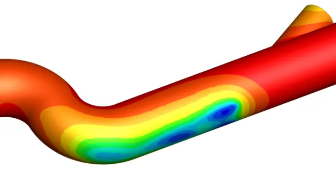
Steady-state pipe wall temperature after pulsed-spray cooling.

Aerospace

One way to achieve higher efficiency in gas turbine engines is to increase the temperatures inside the combustor. These temperatures often exceed the melting point of the metal alloys used to construct gas turbine combustors, necessitating methods for both cooling and insulating the combustor walls. Prediction of the combustor wall temperatures and analyzing various cooling methods include effusion cooling, impingement cooling, and film cooling.

Liquid rockets are another application where capturing CHT is important. As the liquid oxidizer travels from the cryogenic tanks to the combustion chamber, it simultaneously cools the device and picks up heat along the way. The properties of the oxidizer depend on the temperature, often varying from a liquid-like supercritical fluid to a gas-like supercritical fluid, which significantly affects how the oxidizer will mix upon injection into the combustion chamber. Investigating the preheating of the liquid oxidizer is essential for accurately simulating combustion down the line.

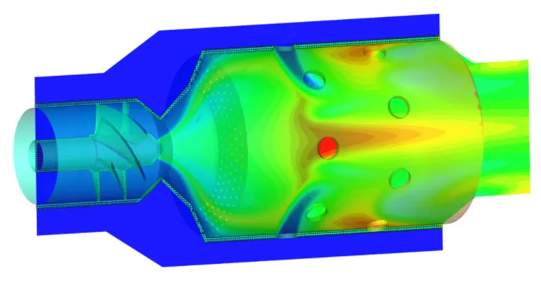
Heat flux through the metal liner of a liquid-fueled gas turbine combustor.

Pumps and Compressors

Resolving the spatially varying surface temperature distributions in pumps and compressors improves the accuracy of the simulation and provides useful temperature data. For example, in a twin screw compressor, thermal expansion affects the clearance between the rotors. If that effect is not captured, the simulations will incorrectly predict leakage flows and lower the accuracy of your results.

Critical Reynolds Number for Flow in a Pipe:

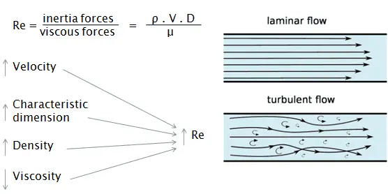
For flow in a pipe of diameter D, experimental observations show that for “fully developed” flow, the critical Reynolds number is about `Re_(d,crit)` = 2300.

Laminar flow: For practical purposes, if the Reynolds number is less than 2000, the flow is laminar. The accepted transition Reynolds number for flow in a circular pipe is `Re_(d,crit)` = 2300.
Transitional flow: At Reynolds numbers between about 2000 and 4000 the flow is unstable as a result of the onset of turbulence. These flows are sometimes referred to as transitional flows.
Turbulent flow: If the Reynolds number is greater than 3500, the flow is turbulent.

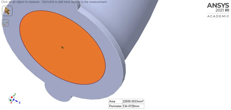
Area =`pi *r^2`
`(22699.0553(mm)^2)/pi = r^2`
`sqrt((22699.0553(mm)^2)/pi) = r`
`r=85.00mm`

Diameter = 170mm

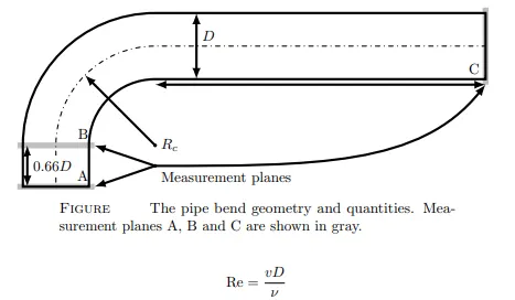
With v being the mean velocity, D is the pipe diameter, and ν is the kinematic viscosity. A pressure outlet boundary condition was imposed on the outlet region and the walls were treated adiabatically with no-slip.

Reynold's number = `(rho*v*d)/mu`
Reynold's number = `(1.225(kg)/(m^3)*5m/s*0.17m)/(1.7894*10^(-5)(kg)/(ms))`= 58,189.89605

It is safe to say that this flow through pipe is a turbulent flow.

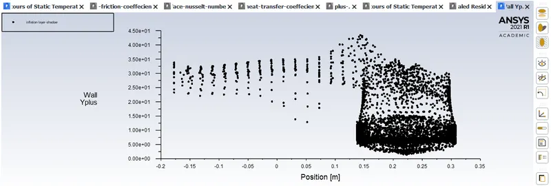
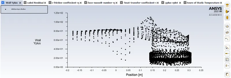
As for what Y+ you need, it depends on the flow of interest and the accuracy you require. It is commonly thought that the SST model requires a small Y+ ( <=1 ), but this is not the case. The SST model is just as accurate as k-epsilon when large Y+ (above 11) are used, in which case it uses a logarithmic wall function to calculate the shear stress at the wall. The advantage to SST is that as you refine the mesh to get closer to the wall, it will transition to a linear wall function and yield more accurate results.

For internal flows, turbulent viscosity ratio of 10-100 it typically a good value

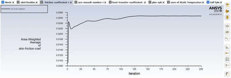
A. Skin friction:

`C_f` = `0.079*Re_D^(-0.25)`

`C_f=0.079*(58189.89605)^(-0.25)`

`C_f=5.08644*10^(-3)`

Alternate formula that can be used when the friction factor is known is given beow:

`ut, two other alternate methods of calculating the skin friction is
1)By using Moody's chart.
2)By using formulas from Heat and mass transfer data book(C P Kothandaraman & S Subramanyan).

1)From Moody's chart: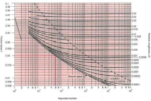

From above for the Reynold's number of 58,189(approximated to 60,000) the friction factor 'f' will be 0.02

where, `C_f` = Skin friction.
`f_D`= Friction factor.

`C_f=0.0205/4=5.125*10^(-3)`

2)Heat and mass transfer data book(C P Kothandaraman & S Subramanyan):

Page 124:

`f=0.184*Re_D^(-0.2)`

`f=0.184*(58189)^(-0.2)`

`f=0.0205`

It must be noted, the skin friction coefficient is equal to the Fanning friction factor. The Fanning friction factor, named after John Thomas Fanning, is a dimensionless number, that is one-fourth of the Darcy friction factor. As can be seen, there is a connection between skin friction forces and frictional head losses.

In turbulent flows, however, things are more difficult, as the friction factor depends strongly on the pipe roughness but here a no slip condition is assumed.

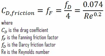
`C_f=0.0205/4=5.126*10^(-3)`

B. Wall shear stress:

The skin friction coefficient is a dimensionless skin shear stress which is nondimensionalized by the dynamic pressure of a free stream.

`C_f=tau_w/((1/2)*rho*v^2)`

where:`C_{f}` is a skin friction coefficient.
`rho` is the density of a fluid.
`v` is the free stream speed, which is the fluid speed far from the body's surface.
`tau_w` is a skin shear stress on a surface.
`(1/2)*rho*v^2` is the dynamic pressure of a free stream.

`tau_w=C_f*((1/2)*rho*v^2)`

`tau_w=(1/2)*5*10^(-3)*1.225((kg)/m^3)*[5(m/s)]^2`

`tau_w=0.0766`

C. Velocity(`U_f`):

`U_f=sqrt((tau_w)/rho)`

`U_f=sqrt((0.0766(kg)/(ms^2))/(1.225(kg)/m^3))`

`U_f=sqrt((0.0766(kg)/(ms^2))/(1.225(kg)/m^3))`

`U_f=2.5m/s`

Here, 4 values of y+ has been considered which are: 30, 50, 100, 200.

For each of these values of y+ a different first layer thickness will be calculated. For w=each first layer thickness a total thickness is calculated based on the number of layers.

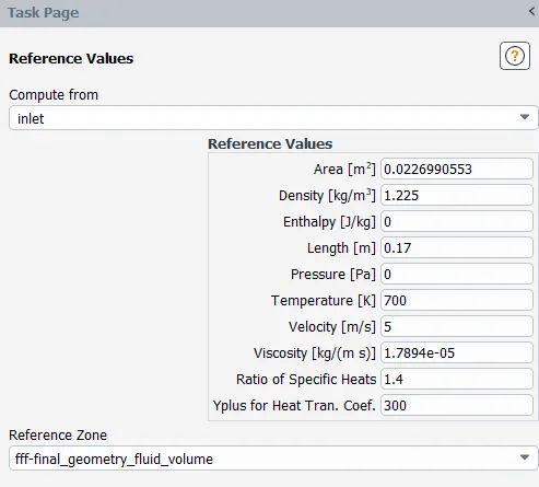
Area in `m^2`: `0.022699m^2`

Charactersitic length = Diameter = 170mm = 0.17m

Steps for setup:

1. Open geometry, import model into spaceclaim.
2. To volume extract,
   Prepare> Volume extract> Edge selection option.
   If you discover duplicate edges
   Repair> extra edges(under fix) > Extra edge >hit the green tick mark.
3. Select both volumes from under structure,(select solid_volume & fluid_volume).
   Right click and choose 'move to a component' & rename it as 'Final geometry'.
   Right click on FFF & select 'delete empty component'.
4. For a clean conformal mesh,
   Go to workbench(from top menu) >Share prep.
   
5. Close spaceclaim and open mesh & update.
6. Under structure, design >volume > rename 'volume' as fluid-volume.
   Under structure, design >volume > rename 'solid' as solid-volume.
   
7. Named selections,
   Select face selection: The 4 circular faces must be named 'inlet'.
   The circular face which is orthogonal to the 4 inlets must be named 'outlet'.
   Double click on the outer wall and name it 'outer-wall-convection'
   Hide the outer envelope(solid-volume).
   Double click on the exterior of the 'fluid-volume'.
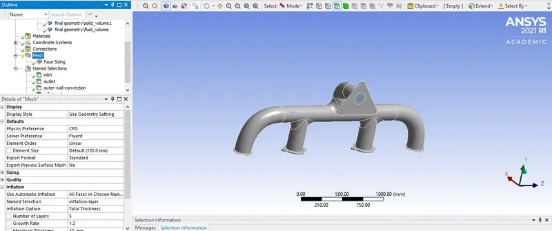
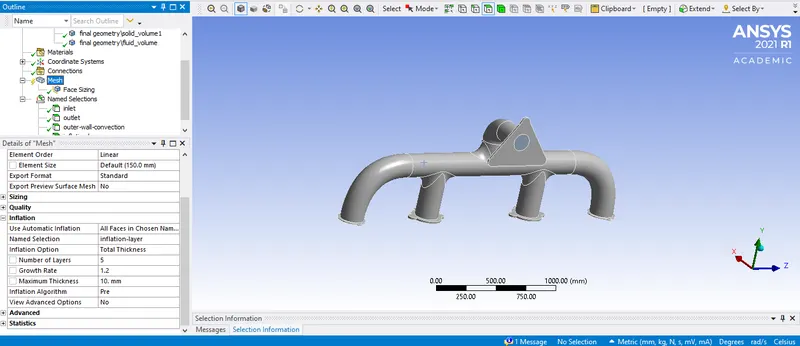
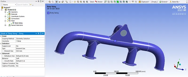
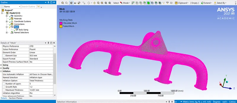
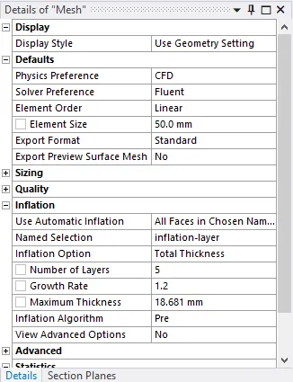
   Name it 'inflation-layer'.
8. Under 'details of mesh', enter element size(50mm).
   Under 'details of mesh', expand 'inflation'
   Change 'Use utomatic inflation' to 'All faces in chosen named selection'.
   'Named selection: Inflation-layer'
   'Inflation option: Total thickness'
   'Number of layers: 5'
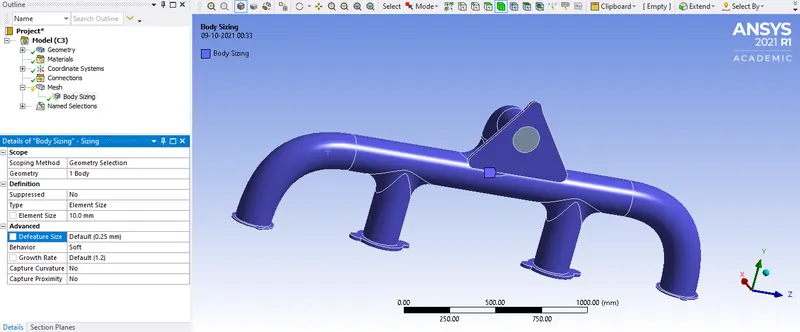
   'Growth rate: 5mm'.
9. Right click on 'mesh' >insert> sizing.
   Under details of face sizing:
   Geometry: select the outer envelope(outer-wall-convection).
   Element size: 100mm
10. Close mesh and update.
11. Open setup,
    Select:
    Pressure based, Steady state solver.
    File> Recorded mesh operations > match zone names.
    Match the geometry to it's appropriate named selection name from mesh interface.
    Domain:
    Display > choose surfaces and hit display to view part & corresponding name.
    Physics:
    Tick 'energy' > viscous model: K-epsilon standard .
    Material: Fluid > air
    : Solid > aluminium > close
    Boundaries(Under zones): Inlet> edit > 5m/s > : Thermal: 700K > ok.
    Zones > Boundaries > outer-wall-convection > edit > thermal condition > select 'convection' > heat transfer coeffecient: 20 > ok.
    Solve:
    Select 'Hybrid' > 'Initialize' the solution.
    Results:
    Graphics > Contours > new > Name: temperature-contour > Contour of: temperature > Surfaces: Inlet, outlet, outer-wall-convection, wall_fff-final-geometry-solid-volume > save/display.
    Solve:
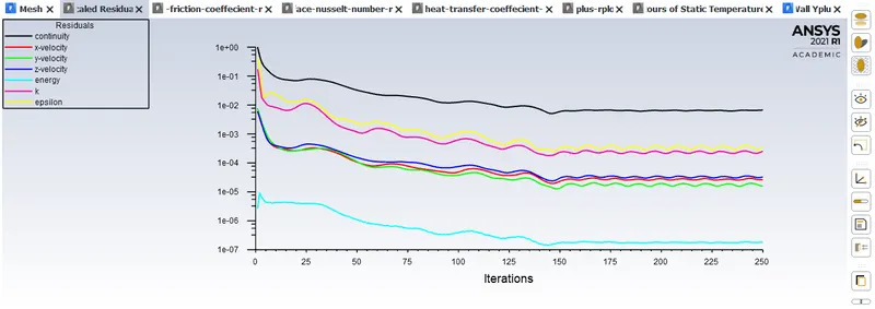
    Run calculation: Number of iterations = 150.
    Activities> create > solution animations > animation object > temperature contour >preview > set the view required > use active > record after :1 > OK.
12. CFD Post: Resultshttps://skill-lync.com/knowledgebase/nusselt-number-2

Baseline simulation:

Mesh element size:

Solid volume: 50mm
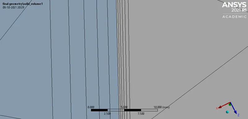
Solid volume inflation layer: 0.7499mm(default)
Fluid volume: 150mm
Fluid volume inflation layer: 10mm(total thickness)

Results:

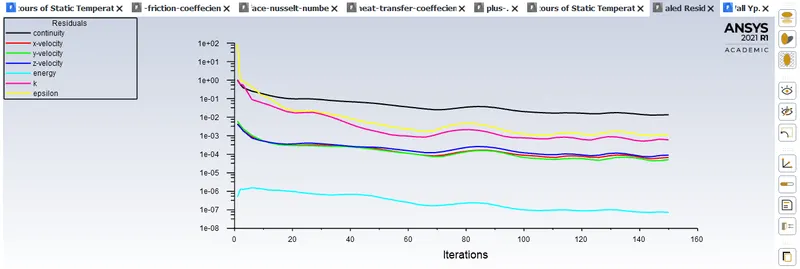
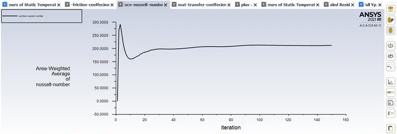
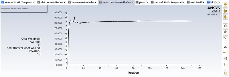
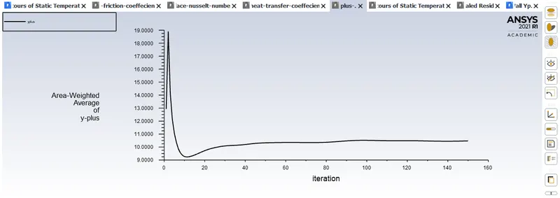
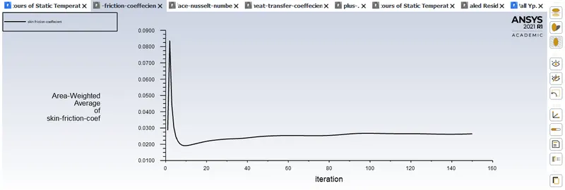
Under 'outline view'
Results > XY Plot

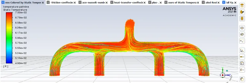
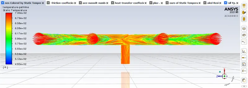
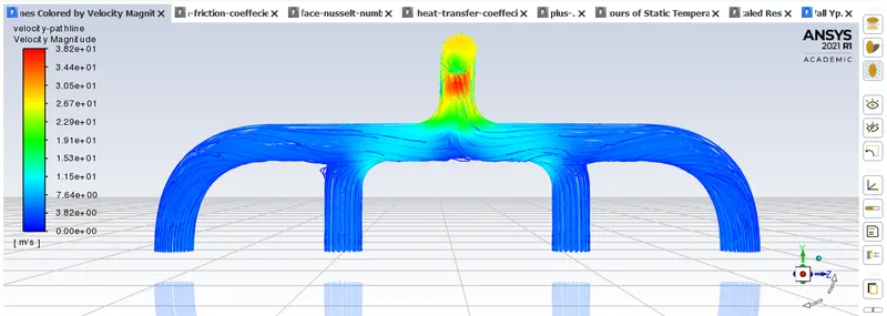
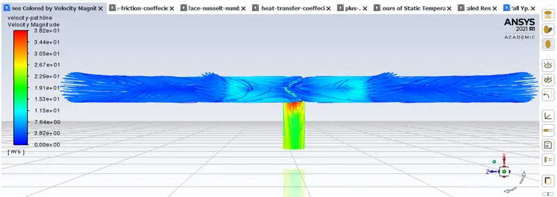
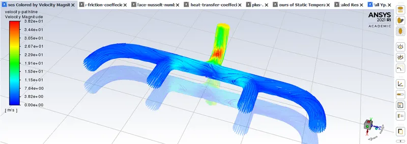
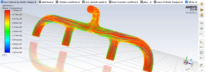
Pathlines:

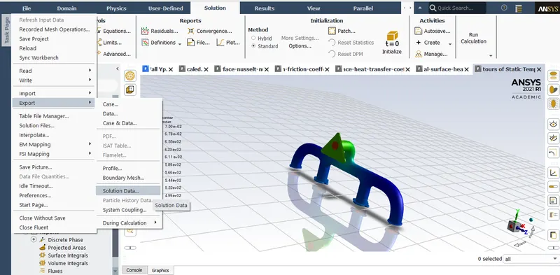
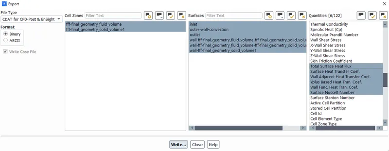
Close setup:

Open Results:

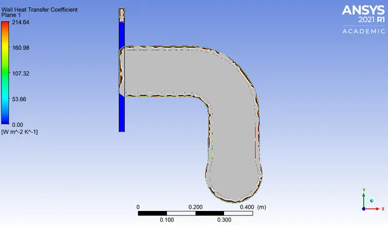
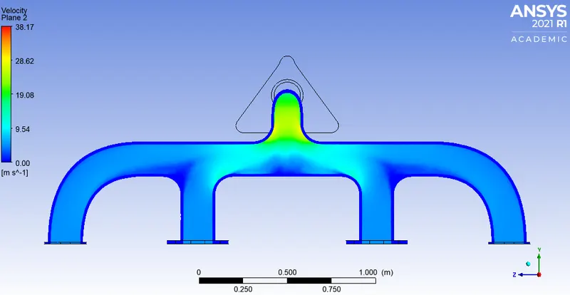
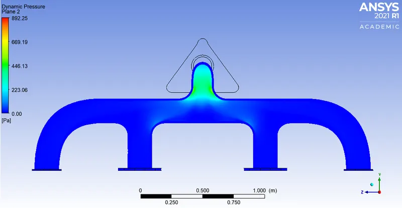
Calculate the wall/surface heat transfer coefficient on the internal solid surface & show the velocity & temperature contours in appropriate areas.

Refined case:

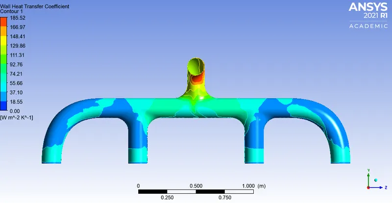
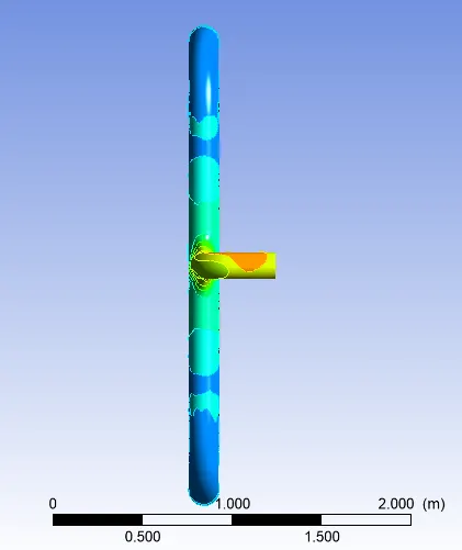
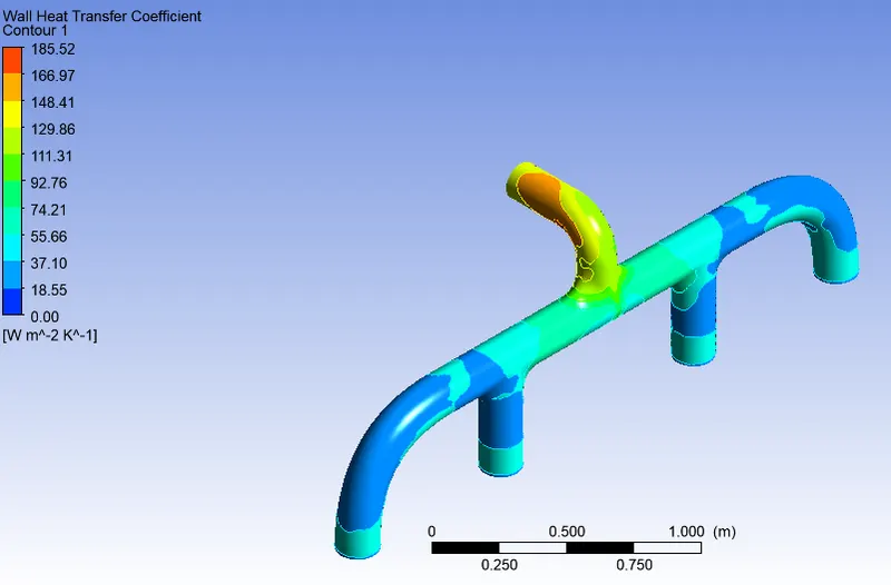
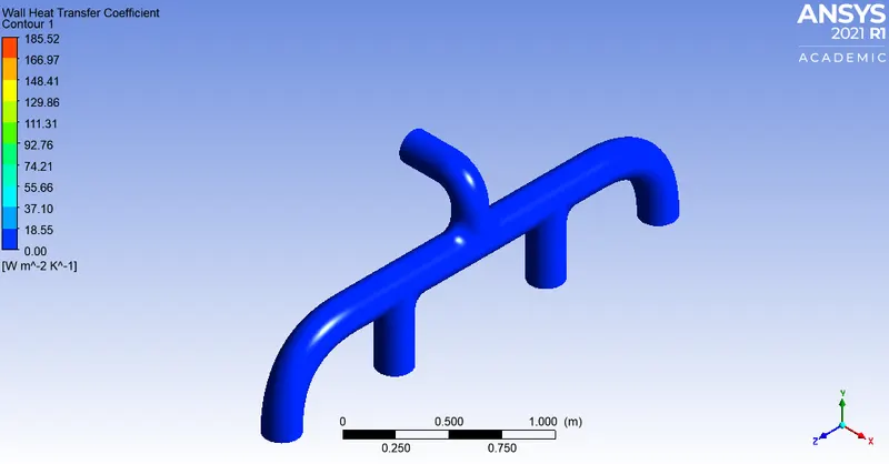
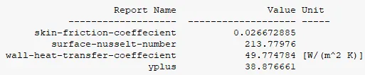
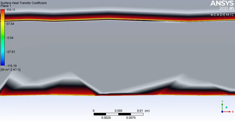
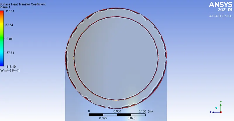
The y+ values influence the results to some extent but however the surface heat transfer coeffecient changes a little bit.

Case 1: y+ = 30,

First layer thickness: 0.17mm

Thickness for y+= 30 :

Since we know that
`U_f`= 2.5m/s,
y+=30,
Density`(rho)` = `1.225(kg)/m^3`
Dynamic viscosity (`mu`) = `1.7894*10^(-5)`

First layer thickness:
`y=(y^+*mu)/(U_f*rho)`
`y=1.7529*10^(-3)m`

For a growth rate of 20% at each successive layer:
Let 'X' be the thickness of the previous layer.
`X+X(20/100)`
Example: `t_2=1.7mm+1.7mm*(20/100)=2.04mm`

t1=1.7mm
t2=1.72.04mm
t3=5.0112mm
t4=5.0112mm
t5=6.0133mm

Total=18.68mm

Mesh configuration:

Solid volume: 100mm
Solid volume inflation layer: 0.5
Fluid volume: 10mm
Fluid volume inflation layer: 12.951mm

Setup:

Steady state: Pressure based solver
Temperature: 700K
Inlet velocity: 5m/s

Plots:

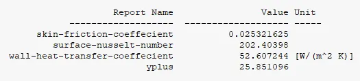
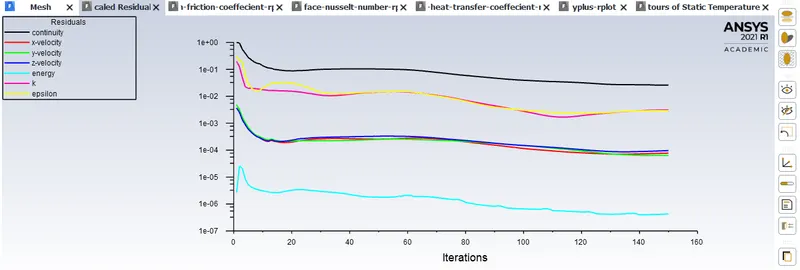
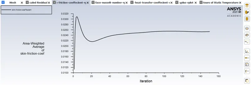
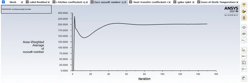
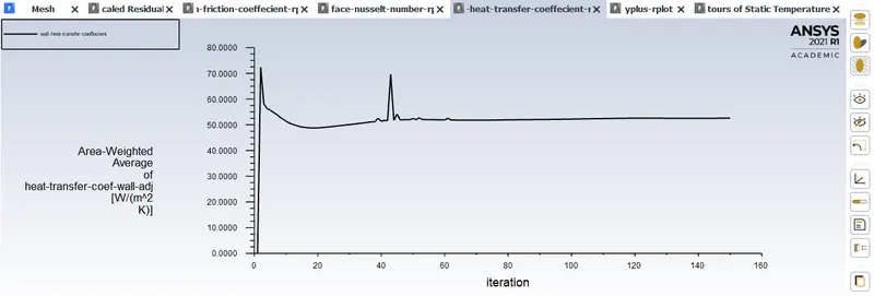
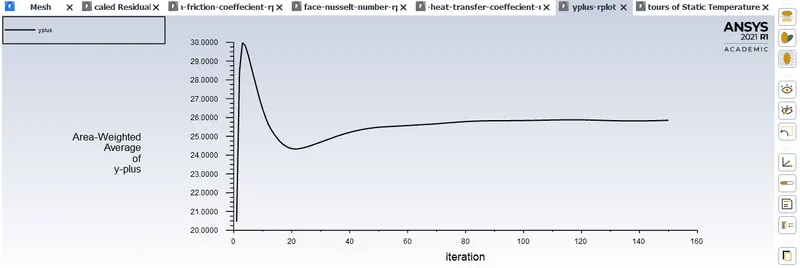
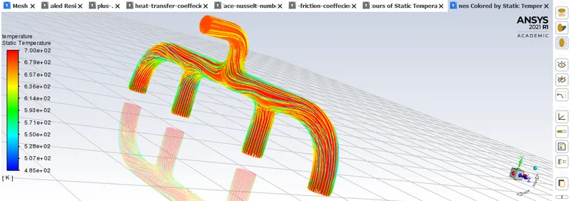
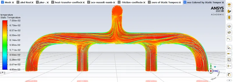
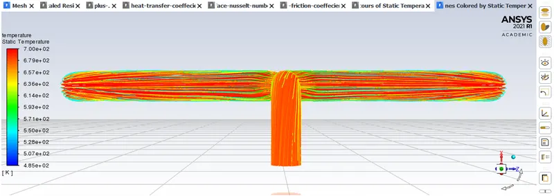
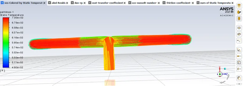
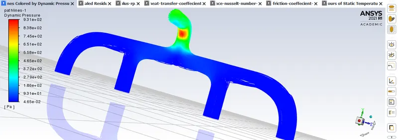
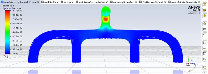
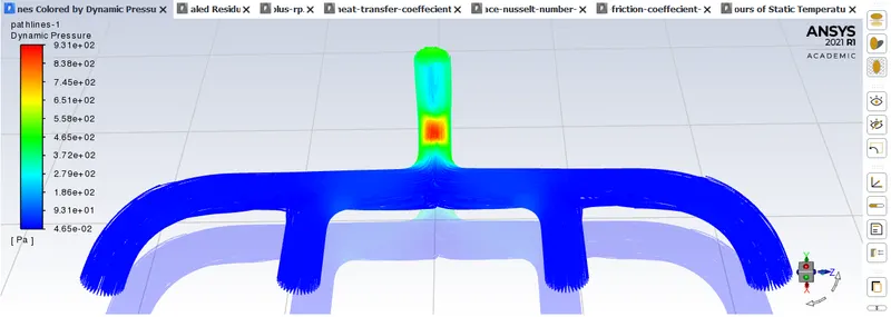
Pathlines:

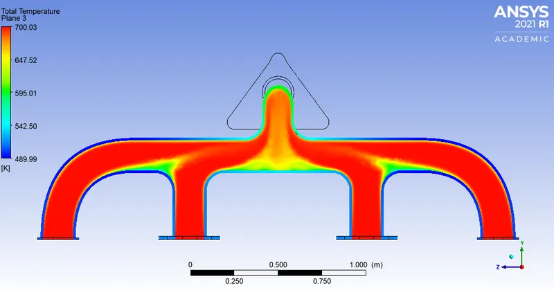
Temperature:

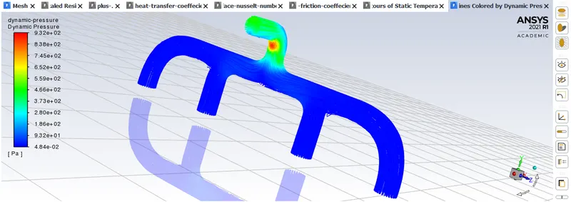
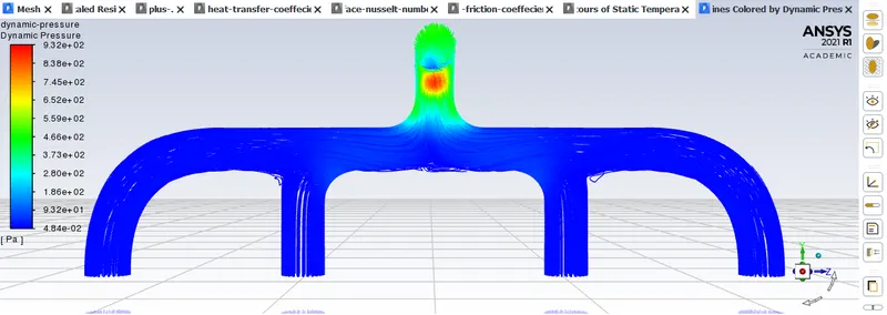
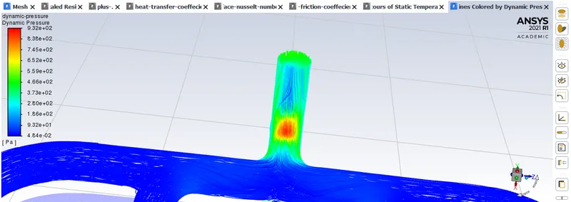
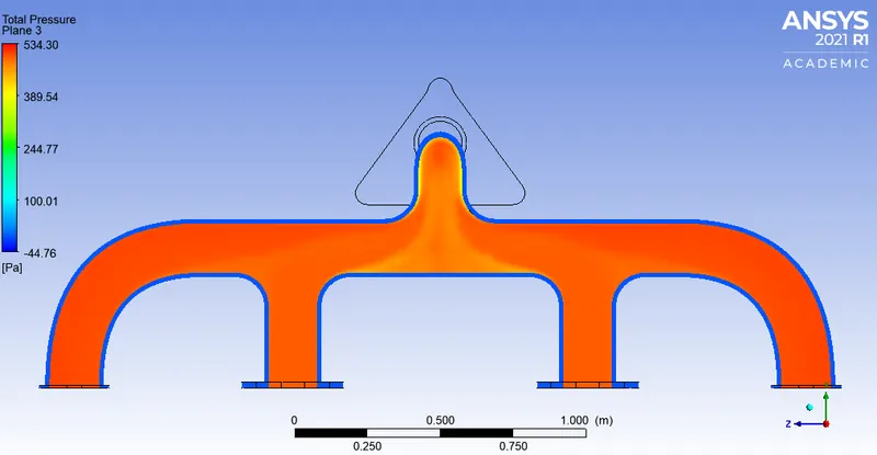
Dynamic pressure:

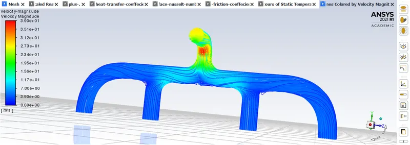
Velocity magnitude:

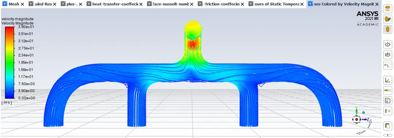
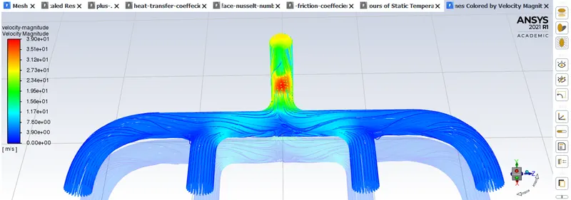
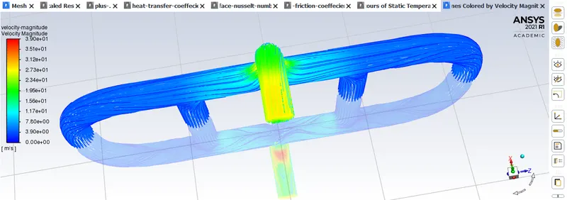
CFD Post: Results

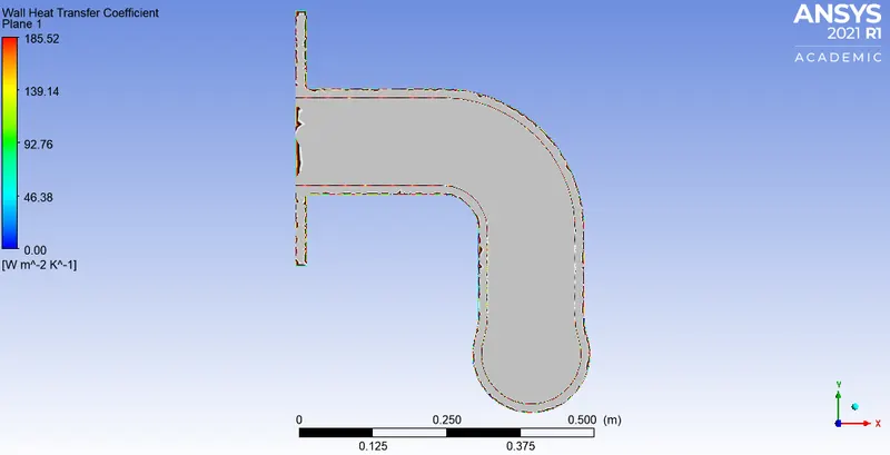
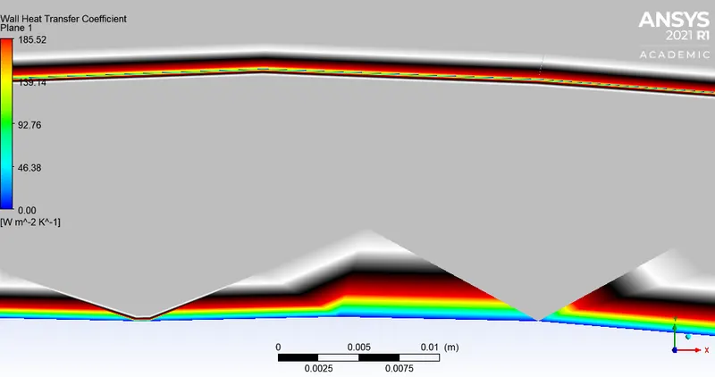
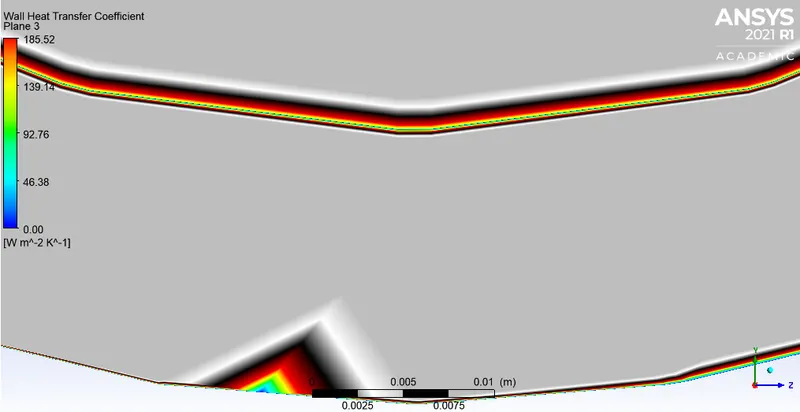
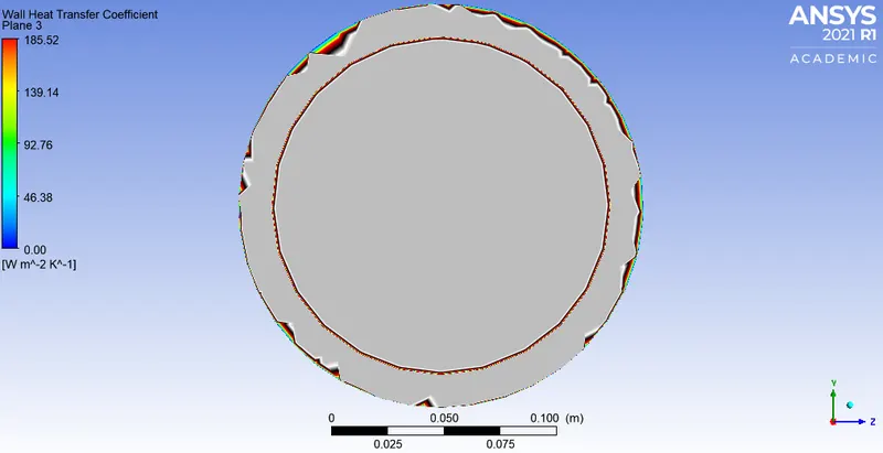
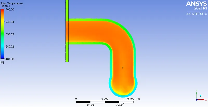
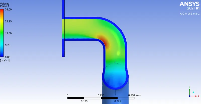
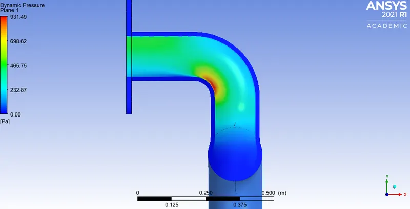
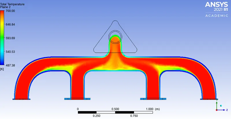
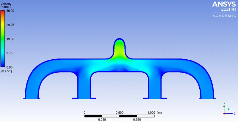
Outer wall

Case 2: y+ = 50

First layer thickness: 2.9mm

Thickness for y+= 50 :

Since we know that
`U_f`= 2.5m/s,
y+=50,
Density`(rho)` = `1.225(kg)/m^3`
Dynamic viscosity (`mu`) = `1.7894*10^(-5)`

First layer thickness:
`y=(y^+*mu)/(U_f*rho)`
`y=2.91*10^(-3)m`

For a growth rate of 20% at each successive layer:
Let 'X' be the thickness of the previous layer.
`X+X(20/100)`
Example: `t_2=2.9mm+2.9mm*(20/100)=3.48mm`

t1=2.9mm
t2=3.48mm
t3=4.176mm
t4=5.0112mm
t5=6.0133mm

Total=18.68mm

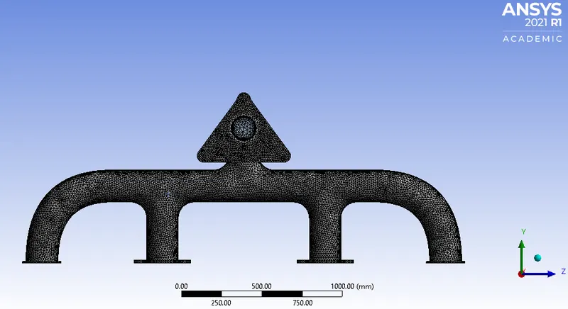
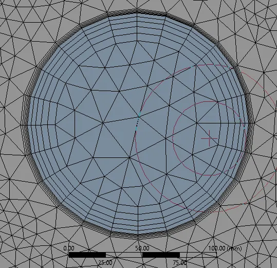
Mesh configuration:

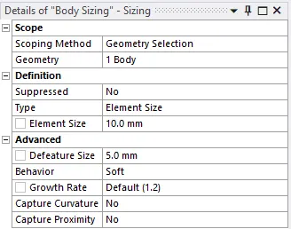
Solid volume: 10mm
Solid volume inflation layer: 5mm
Fluid volume: 50mm
Fluid volume inflation layer: 18.681mm

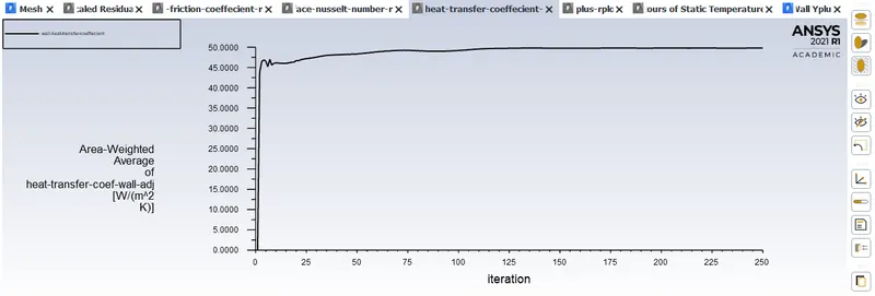
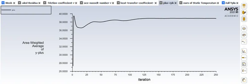
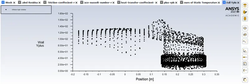
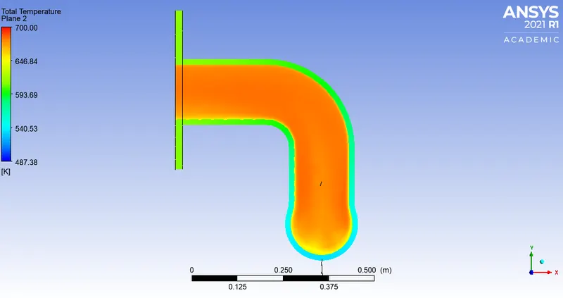
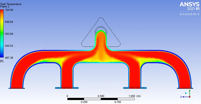
Temperature:

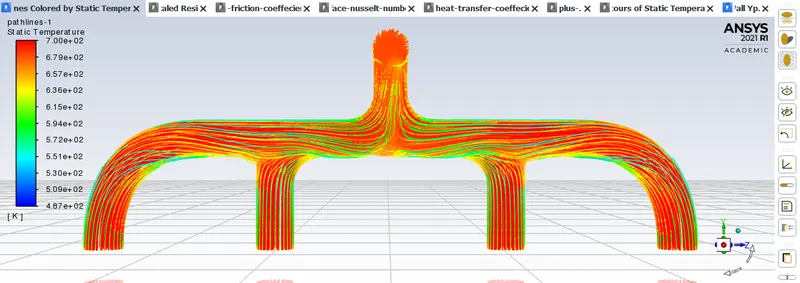
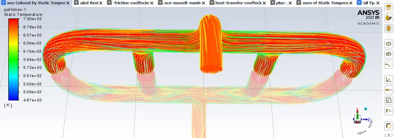
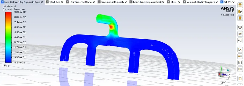
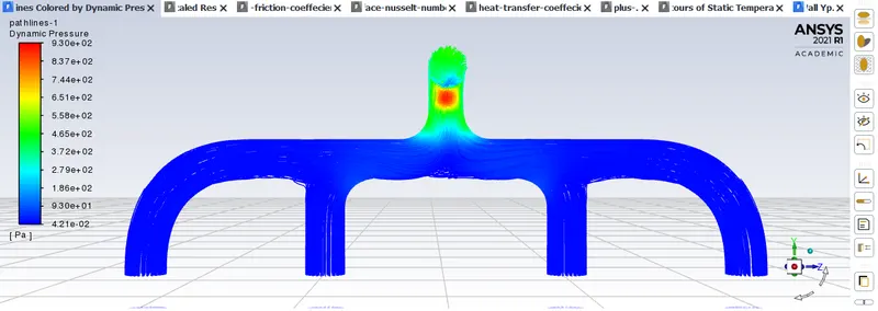
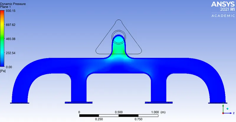
Static pressure:

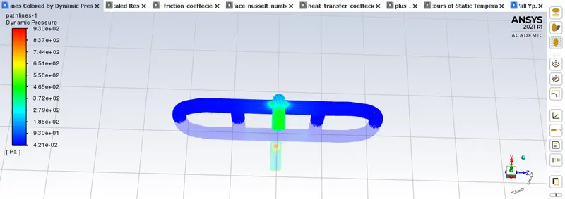
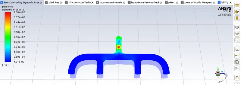
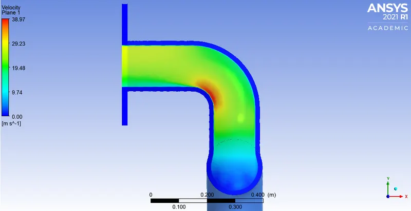
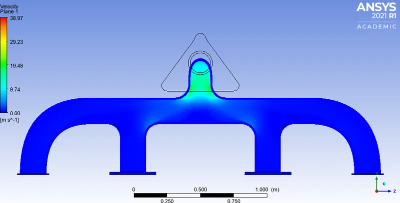
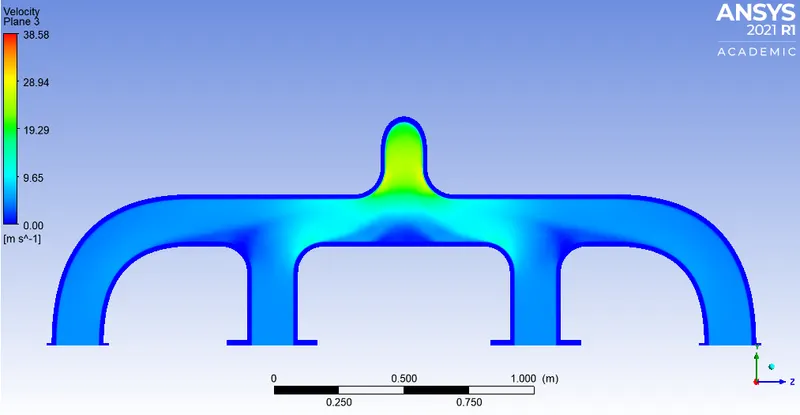
Velocity:

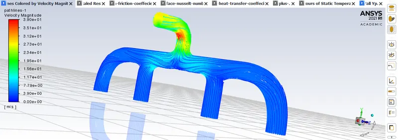
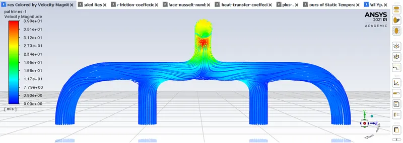
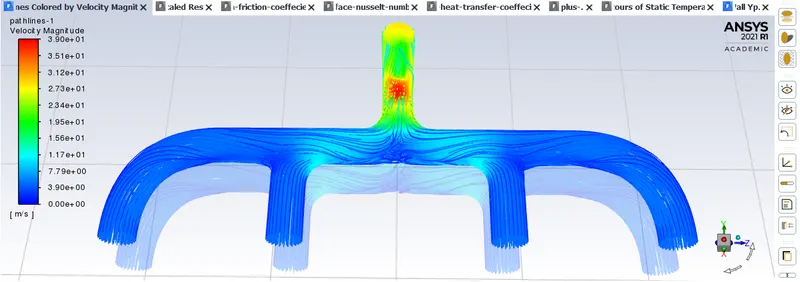
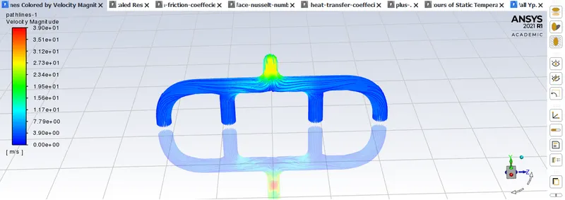
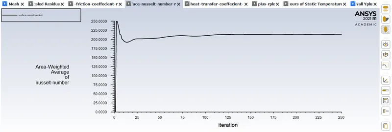
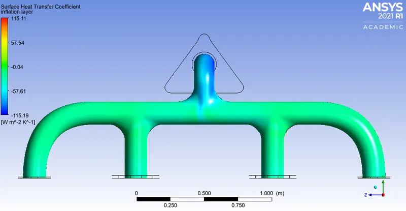
CFD Post/Results:

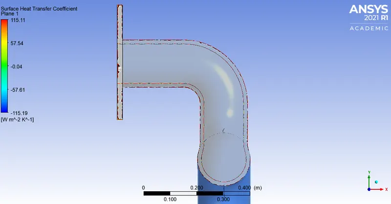
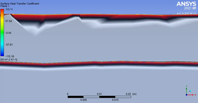
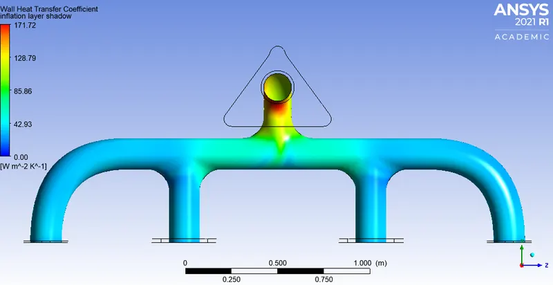
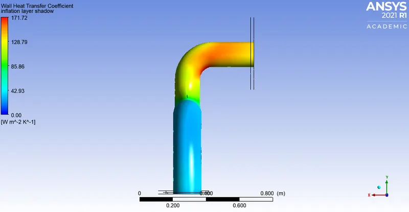
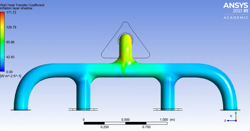
Case 3: y+ = 100

First layer thickness: 5.8mm

Thickness for y+= 100 :

Since we know that
`U_f`= 2.5m/s,
y+=100,
Density`(rho)` = `1.225(kg)/m^3`
Dynamic viscosity (`mu`) = `1.7894*10^(-5)`

First layer thickness:
`y=(y^+*mu)/(U_f*rho)`
`y=5.8428*10^(-3)m`

For a growth rate of 20% at each successive layer:
Let 'X' be the thickness of the previous layer.
`X+X(20/100)`
Example: `t_2=5.8mm+5.8mm*(20/100)=6.96mm`

t1=5.8mm
t2=6.96mm
t3=8.352mm
t4=10.0224mm
t5=12.0269mm

Total=43.16128mm

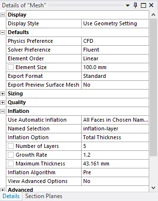
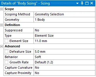
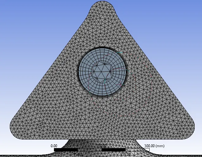
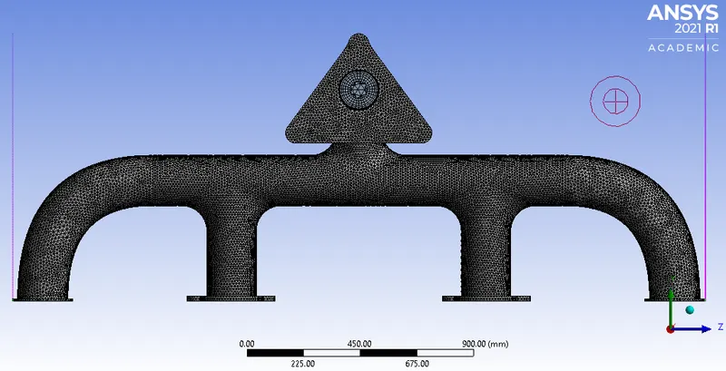
Solid volume: 11mm
Solid volume inflation layer: 5mm
Fluid volume: 100mm
Fluid volume inflation layer: 43.16128mm

Setup:

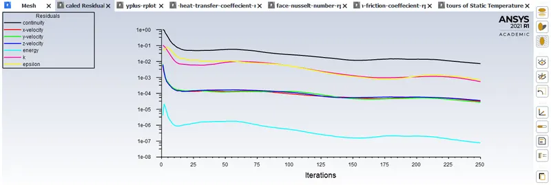
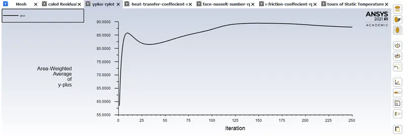
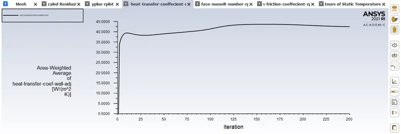
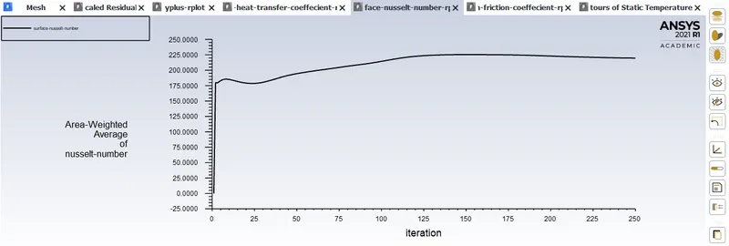
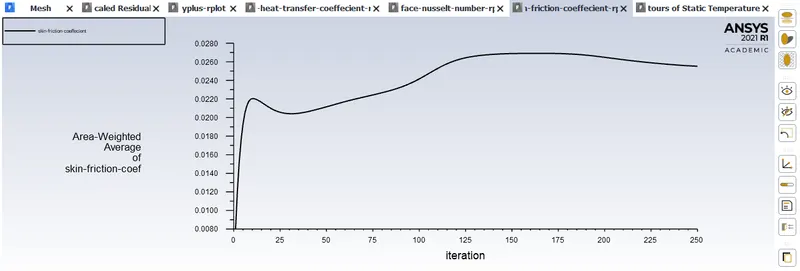
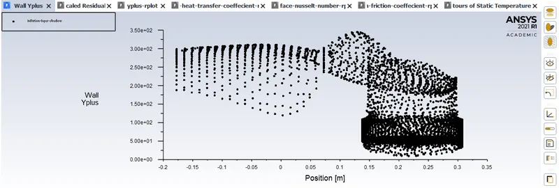
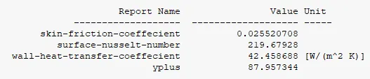
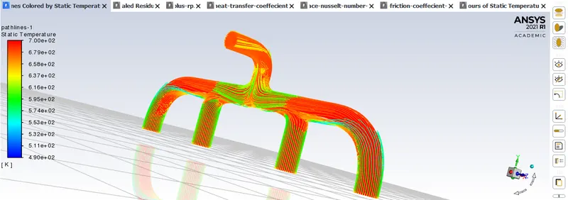
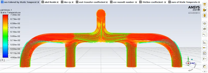
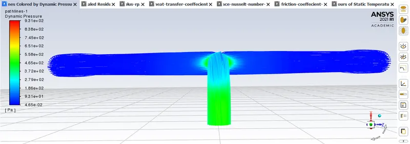
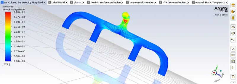
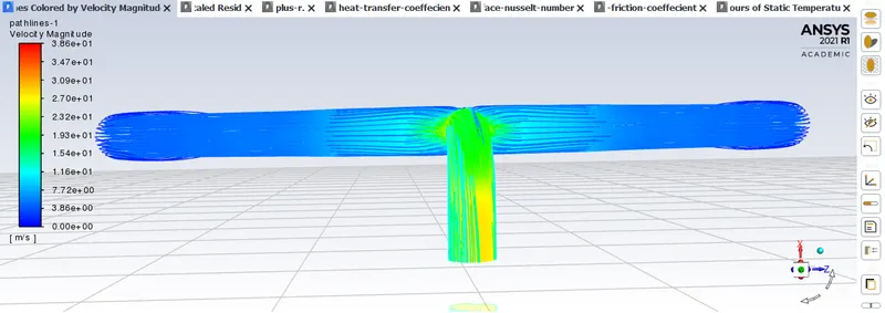
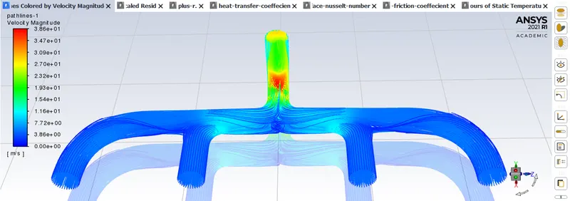
CFD Post: Results

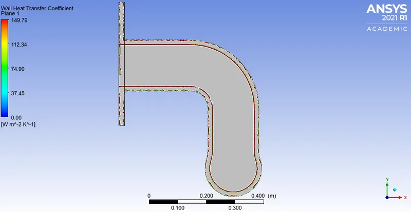
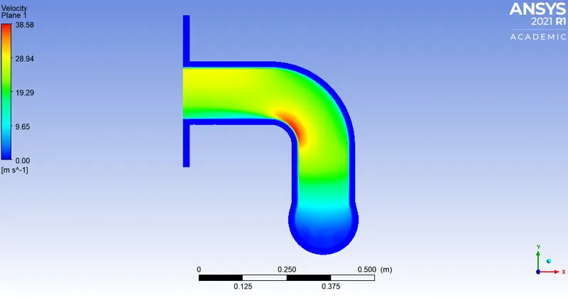
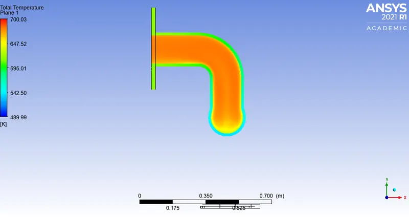
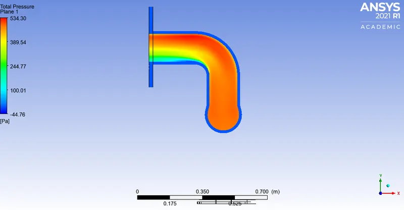
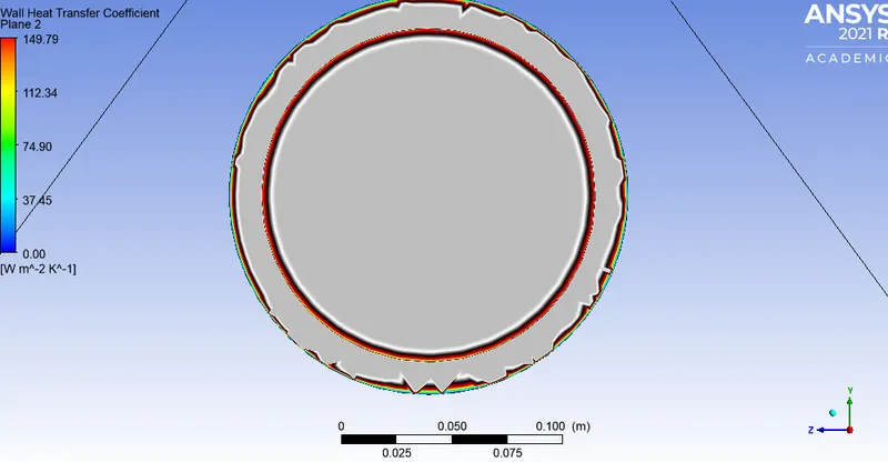
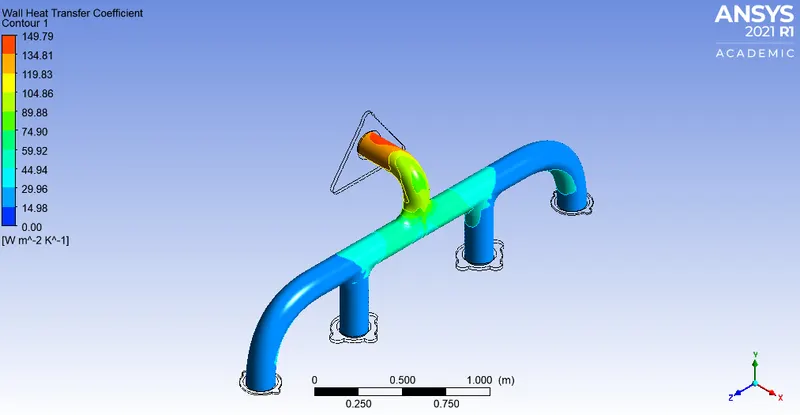
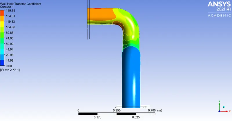
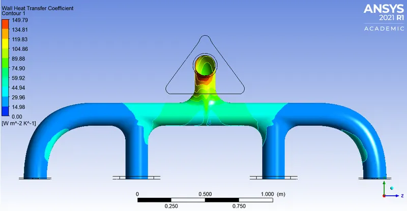
Surface heat transfer coeffecient:

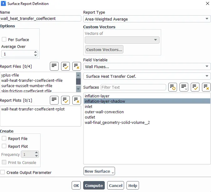
y+: 30

y+: 50

y+: 100

Analytical verification for surface heat transfer coeffecient:

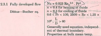
Page 125: Heat and mass transfer data handbook(C P Kothandaraman & S Subramanyan).

Reynold's number = `(rho*v*d)/mu`
Reynold's number = `(1.225(kg)/(m^3)*5m/s*0.17m)/(1.7894*10^(-5)(kg)/(ms))`= 58,189.89605

Prandlt number: Pr = The ratio of momentum diffusivity to thermal diffusivity.

where:

• `nu` : momentum diffusivity (kinematic viscosity), `nu=mu/rho`, (SI units: m²/s)
• `alpha` : thermal diffusivity, `alpha=k/(rho*C_p)`, (SI units: m²/s)
• `mu` : dynamic viscosity, (SI units: Pa s = N s/m²) = 1.7894*10^(-5)(kg)/(ms)
• `k` : thermal conductivity, (SI units: W/(m·K))= 0.024W/(m·K),(air, `(kg⋅m)/(s^(3)*K)`
• `C_p` : specific heat, (SI units: J/(kg·K)) = 1007 (m^3/s^2*K)
• `rho` : density, (SI units: kg/m³) = 1.225kg/m³.

Pr=`(1007m^3/(s^2*K)*(1.7894*10^(-5)(kg)/(ms)))/[0.024[(kg⋅m)/(s^(3)*K)]]`

= 0.7508

So, Nusselt's number = `0.023*Re^0.8Pr^0.4`
= `0.023*(58190)^(0.8)*(0.7508)^0.4`
= 132.98

But, Nusselt's number = hL/(k)
L=Characteristic length=Diameter of the inlet=0.17m

h=k*Nu/L

h=18.77W/(m²•K)

The change in velocity at the the throat near the outlet is because of convservation of mass. The exhasut gases entering from the inlet causes this increase in velocity at the outlet.

Factors affecting accuracy:

1. Mesh:
The mesh must be coarse enough with additional features such as inflation layers, this helps the software to approximate better values neat the boundaries and the walls. The mesh need not be too coarse because it will be computationally expensive without any significant change in the results.

2. y+ value:
The y+ values are very important when it comes to capturing the fluid interaction and it's effect on the boundaries. Large values of y+ produce less accurate results when compared to lower y+ values. A particular value of y+ requires a certain turbulence model for calculations.

3. Turbulence model:
Appropriate turbulence model which satisfy the y+ value must be chosen.
Y+ : 0 to 30 : K-Omega model.
Y+ : 30 to 300 : K-epsilon model.

REFERENCES:

Conjugate heat transfer:

https://convergecfd.com/benefits/conjugate-heat-transfer

https://www.simscale.com/docs/analysis-types/conjugate-heat-transfer-analysis/

Skin friction:

https://www.thermal-engineering.org/what-is-skin-friction-friction-drag-definition/

https://en.wikipedia.org/wiki/Skin_friction_drag

y+:

https://www.computationalfluiddynamics.com.au/tips-tricks-cfd-estimate-first-cell-height/

y+ tutorial:

https://www.youtube.com/watch?v=4lPwgQ59VT0

y+ calculator:

https://www.cfd-online.com/Tools/yplus.php

Table of quantities:
https://www.engineersedge.com/physics/viscosity_of_air_dynamic_and_kinematic_14483.htm