Week 6 - Multivariate Newton Rhapson Solver
Newton raphson method : Single variable
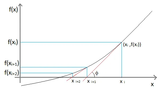
Slope of the first tangent = `tan(phi)=(Deltay)/(Deltax)`
= `tan(phi)=(f(x_i)-0)/(x_i-x_(i+1))`
But ,`tan(phi)`= `f'(x_i)`
So ,`f'(x_i)=(f(x_i)-0)/(x_i-x_(i+1))`
`x_(i+1)=x_i-f(x_i)/( f'(x_i))`
For multivariate newton raphson method ,the `f'(x_i)`can be replaced with a Jacobian matrix .
This Jacobian matrix contains the derivatives of each function with respect to the number of variables in the non linear system ,so it is safe to say that we can use the Jacobian in place of `f'(x_i)`.
Also the function in the multivariate newton raphson method will contain more than one variable so we can replace `f(x_i)` with F .
`F= ((f_1),(f_2),(.),(.),(.),(f_n))`
Equation for Multivariate Newton Method : (We have changed the variables from 'x' to `(y_1,y_2,y_3,....,y_n)`
`Y_(i+1)=Y_i-f/( J)`
Taking the inverse of the Jacobian
`Y_(i+1)=Y_i-J^(-1)f`
We can introduce the relaxation factor `(alpha)` to the above equation ,
`Y_(i+1)=Y_i-(alpha)J^(-1)f`
where,
`J=[[(delf_1)/(dely_1) ,(delf_1)/(dely_2) ,(delf_1)/(dely_3),.,.,.,(delf_1)/(dely_n)],[(delf_2)/(dely_1),(delf_2)/(dely_2),(delf_2)/(dely_3),.,.,.,(delf_2)/(dely_n)],[(delf_3)/(dely_1),(delf_3)/(dely_2),(delf_3)/(dely_3),.,.,.,(delf_1)/(dely_n)],[.,.,.,.,.,.,.],[.,.,.,.,.,.,.],[(delf_n)/(dely_1) ,(delf_n)/(dely_2) ,(delf_n)/(dely_3),.,.,.,(delf_n)/(dely_n)]]`
`F= [(f_1(x1,x2,x3,..x_n)),(f_2(x1,x2,x3,..x_n)),(.),(.),(.),(f_n(x1,x2,x3,..x_n))]`
`Y_(i+1)=Y^(n ew) =[(Y^(1,n ew)),(Y^(2,n ew)),(Y^(3,n ew)),(.),(.),(.),(Y^(n,n ew))]`
`Y_(i)=Y^(old) =[(Y^(1,old)),(Y^(2,old)),(Y^(3,old)),(.),(.),(.),(Y^(n,old))]`
Given non linear equations :
`(dy_1)/dt = -0.004*y_1+10^4*y_2*y_3`
`(dy_2)/dt = 0.04*y_1-10^4*y_2*y_3-3*10^7*y_2^2`
`dy_3/dt = 3*10^7*y_2^2`
Applying Newton raphson for a system of coupled non-linear equations .
`Y_(i+1)=Y_i-(alpha)J^(-1)f`
where,
`Y^(n ew) =[(Y^(1,n ew)),(Y^(2,n ew)),(Y^(3,n ew))]`
`Y^(old) =[(Y^(1,old)),(Y^(2,old)),(Y^(3,old))]`
`J=[[(delf_1)/(dely_1) ,(delf_1)/(dely_2) ,(delf_1)/(dely_3)],[(delf_2)/(dely_1),(delf_2)/(dely_2),(delf_2)/(dely_3)],[(delf_3)/(dely_1),(delf_3)/(dely_2),(delf_3)/(dely_3)]]`
`F= ((f_1(y1,y2,y3)),(f_2(y1,y2,y3)),(f_3(y1,y2,y3)))`
Stability of euler backward differencing :
From taylor's series expansion
`f(x+a)=f(x)+(d[f(x)])/(dx)*Deltax+(d^2[f(x)])/(dx^2)*(Deltax^2)/(2!)+(d^3[f(x)])/(dx^3)*(Deltax^3)/(3!)+........`
Ignoring higher order terms and rearranging the equation ,
`(d[f(x)])/(dx)=f((x+a)-f(x))/(Deltax)`
Now consider an ODE ,
`y'=f(t,y)`
or
`(d(y))/dt=f(t,y(t))`
and the initial condition being `y(t_0)=y_0`
To numerically approximate a first order ODE with the Backward Euler (BE) method, we make the following approximation of the first derivative term:
`(d(y))/dt=(y_n-y_(n-1))/(Deltat)`
also,
`(y_n-y_(n-1))/(Deltat)=f(t_n,y_n)`
Here we are determining the slope of the point behind out reference point "n" .
By changing our reference point from "n" to "n+1" we get the following equation :
`(y_(n+1)-y_(n))/(Deltat)=f(t_(n+1),y_(n+1))`
Futhermore ,
`y_(n+1)=y_(n)+[f(t_(n+1),y_(n+1))]*(Deltat)`
Let `[f(t_(n+1),y_(n+1))]=y'=-lambday` & `y_0=1;t>=0;lambda>0`
The equation becomes the following when we substitute the above conditions ,
`y_(n+1)=y_(n)-hlambda*y_(n+1)*(Deltat)`
`(1+hlambda*Deltat)*y_(n+1)=y_(n)`
`y_(n+1)=(1/((1+hlambda*Deltat)))y_(n)`
For stability we need :
`|(1)/(1+hlambda*Deltat)|<1` which is true for any value of "h" ie., h>0
Hence the implicit method is "Absolutely stable"
&
For us to be able to solve an Implicit Euler's formula by using the Newton Raphson method equate the whole equation to zero .
`y_(n)-y_(n+1)+[f(t_(n+1),y_(n+1))]*(Deltat)=0`
Problem origin :
This problem originates from the Akzo Nobel Central Research in Arnhem, the Netherlands.
It describes a chemical process in which two species, FLB and ZLU, are mixed while carbon dioxide is continuously added. The resulting species of importance is ZLA . The reaction equations are given
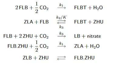
The last equation describes an equilibrium where the constant
`K_s=[[FLB.ZHU]]/([FLB]·[ZHU])`
Robertson problem :
The following equations are a part of a kinetics problem, given by Robertson, is frequently used as an illustrative example. It involves the following three nonlinear rate equations:
`A rightarrow^(k1) B`
`B + B rightarrow^(k2) C + B`
`B + C rightarrow^(k3) A + C`
The problem describes the kinetics of an autocatalytic reaction given by Robertson (1966)
Here k1, k2, k3 are the rate constants and A, B and C are the chemical species involved. Under some idealized conditions and the assumption that the mass action law is applied for the rate functions, the following mathematical model consisting of a set of three ODEs can be set up
`((y_1^'),(y_2^'),(y_3^'))=((−k_1y_1 + k_3y_2y_3),(k_1y_1 − k_2y_2^2 − k_3y_2y_3),(k_2y^2))` with `(y_1(0), y_2(0), y_3(0))^T= (y_(01), y_(02), y_(03))^T`
where y1, y2, y3 denote the concentrations of A, B and C respectively and `y_(01), y_(02), y_(03)` are the concentrations at time t = 0. Here we will be running the code for 600seconds(10 mins) as required.
The problem is very popular in numerical studies and it is often used as a test problem in the stiff integrators comparisons. The numerical values of the rate constants used in the test problem are `k_1 = 0.04`, `k_2 = 3 · 10^7` and `k_3 = 10^4`.
The initial concentrations y01 = 1, y02 =0, y03 = 0. The large difference among the reaction rate constants is the reason for stiffness. As is typical for problems arising in chemical kinetics this special system has a small very quick initial transient. This phase is followed by a very smooth variation of the components where a large stepsize would be appropriate for a numerical method.
By substituting the values for `(k_1,k_2,k_3)` ,we get
`dy_1/(dt)=-0.04y_1+10^4y_2y_3`
`dy_2/(dt)=-0.04y_1-10^4y_2y_3-3*10^7y_2^2`
`dy_3/(dt)=3*10^7y_2^2`
The above equations can be equated to zero in the following way .
`[y1_(n+1)-y1_(n)]/(Deltat)= 10^4*y2*y3 - 0.04*y1`
`[y2_(n+1)-y2_(n)]/(Deltat)=0.04*y1 - 10^4*y2*y3 - 3*10^7*y2^2`
`[y3_(n+1)-y3_(n)]/(Deltat)=3*10^7*y2^2`
Now for us to be able to execute Newton-Raphson method on the above equations ,
`y1_n + (10^4*y2*y3 - 0.04*y1)*dt - y1_(n+1) =0`
`y2_(n) + (0.04*y1 - 10^4*y2*y3 - 3*10^7*y2^2)*dt - y2_(n+1)=0`
`y3_n + (3*10^7*y2^2)*dt - y3_(n+1)=0`
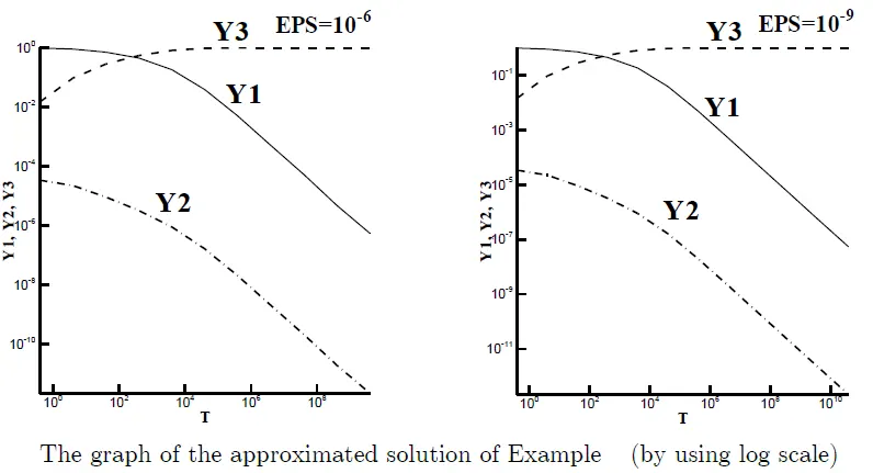
Expected trend :
Code :
import numpy as np
import matplotlib.pyplot as plt
from numpy.linalg import inv

def f1(y1_prev,y1,y2,y3,dt):

	return y1_prev + (10**4*y2*y3 - 0.04*y1)*dt - y1

def f2(y2_prev,y1,y2,y3,dt):

	return y2_prev + (0.04*y1 - 10**4*y2*y3 - 3*10**7*y2**2)*dt - y2

def f3(y3_prev,y1,y2,y3,dt):

	return y3_prev + (3*10**7*y2**2)*dt - y3


def jacobian(y1_prev,y2_prev,y3_prev,y1,y2,y3,dt):
	"""Populating the Jacobian matrix"""

	J=np.ones((3,3))
	delta=1e-4                      # spatial

	J[0,0]=(f1(y1_prev,y1+delta,y2,y3,dt)-f1(y1_prev,y1,y2,y3,dt))/delta
	J[0,1]=(f1(y1_prev,y1,y2+delta,y3,dt)-f1(y1_prev,y1,y2,y3,dt))/delta
	J[0,2]=(f1(y1_prev,y1,y2,y3+delta,dt)-f1(y1_prev,y1,y2,y3,dt))/delta

	J[1,0]=(f2(y2_prev,y1+delta,y2,y3,dt)-f2(y2_prev,y1,y2,y3,dt))/delta
	J[1,1]=(f2(y2_prev,y1,y2+delta,y3,dt)-f2(y2_prev,y1,y2,y3,dt))/delta
	J[1,2]=(f2(y2_prev,y1,y2,y3+delta,dt)-f2(y2_prev,y1,y2,y3,dt))/delta

	J[2,0]=(f3(y3_prev,y1+delta,y2,y3,dt)-f3(y3_prev,y1,y2,y3,dt))/delta
	J[2,1]=(f3(y3_prev,y1,y2+delta,y3,dt)-f3(y3_prev,y1,y2,y3,dt))/delta
	J[2,2]=(f3(y3_prev,y1,y2,y3+delta,dt)-f3(y3_prev,y1,y2,y3,dt))/delta

	return J

y1_prev=1
y2_prev=0
y3_prev=0

#numpy column vector
y_prev=np.ones((3,1))

y_prev[0]=y1_prev
y_prev[1]=y2_prev
y_prev[2]=y3_prev

#numpy column vector for F
F=np.copy(y_prev)

#parameters for newton raphson solver
alpha=1

#time loop
total_t=600
dt=0.1
n=int(total_t/dt)
t_array=np.arange(0,n,dt)


#starting NR loop
iter=1

y_new_array_one=[]
y_new_array_two=[]
y_new_array_three=[]
iter_array=[]
sum_array=[]

for i in range(0,n):

	tol=1e-2
	#initial error
	error=9                                #can use any positive integer

	while error>tol:

		J=jacobian(y_prev[0],y_prev[1],y_prev[2],y1_prev,y2_prev,y3_prev,dt)

		#computing the F vector old values are used
		F[0]=f1(y1_prev,y_prev[0],y_prev[1],y_prev[2],dt)
		F[1]=f2(y2_prev,y_prev[0],y_prev[1],y_prev[2],dt)
		F[2]=f3(y3_prev,y_prev[0],y_prev[1],y_prev[2],dt)

		#computing new values
		y_new=y_prev-alpha*np.matmul(inv(J),F)

		#computing max absolute error
		error=np.max(np.abs(y_new-y_prev))


		add=y_new[0]+y_new[1]+y_new[2]
		sum_array.append(add)

		#updating old values

		y_prev=y_new                                                  #solution update

	#log message
	log_message = 'iteration # = {0} y1={1} y2={2} y3={3}'.format(iter,y_prev[0],y_prev[1],y_prev[2])
	print(log_message)

	iter=iter+1

	y_new_array_one.append(y_new[0])
	y_new_array_two.append(y_new[1])
	y_new_array_three.append(y_new[2])
	iter_array.append(iter)

	y1_prev=y_new[0]
	y2_prev=y_new[1]
	y3_prev=y_new[2]


plt.plot(iter_array,y_new_array_one)
plt.xlabel('Iteration number')
plt.ylabel('Y 1')
plt.show()
plt.plot(iter_array,y_new_array_two)
plt.xlabel('Iteration number')
plt.ylabel('Y 2')
plt.show()
plt.plot(iter_array,y_new_array_three)
plt.xlabel('Iteration number')
plt.ylabel('Y 3')
plt.show()

plt.plot(iter_array,y_new_array_one,label='Y1')
plt.plot(iter_array,y_new_array_two,label='Y2')
plt.plot(iter_array,y_new_array_three,label='Y3')
plt.legend()
plt.title('Y values in a log plot')
plt.yscale("log")
plt.xscale("log")
plt.xlabel('Iteration number')
plt.ylabel('Y values')
plt.show()

plt.plot(iter_array,sum_array)
plt.title('The sum of y1 ,y2 & y3 at each iteration')
plt.yscale("log")
plt.show()
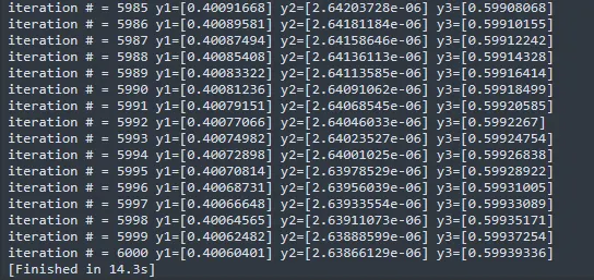
Code : With descriptive print statements about function input values .
import numpy as np
import matplotlib.pyplot as plt
from numpy.linalg import inv

def f1(y1_prev,y1,y2,y3,dt):

	return y1_prev + (10**4*y2*y3 - 0.04*y1)*dt - y1

def f2(y2_prev,y1,y2,y3,dt):

	return y2_prev + (0.04*y1 - 10**4*y2*y3 - 3*10**7*y2**2)*dt - y2

def f3(y3_prev,y1,y2,y3,dt):

	return y3_prev + (3*10**7*y2**2)*dt - y3


def jacobian(y1_prev,y2_prev,y3_prev,y1,y2,y3,dt):
	"""Populating the Jacobian matrix"""

	J=np.ones((3,3))
	delta=1e-4                      # spatial

	J[0,0]=(f1(y1_prev,y1+delta,y2,y3,dt)-f1(y1_prev,y1,y2,y3,dt))/delta
	J[0,1]=(f1(y1_prev,y1,y2+delta,y3,dt)-f1(y1_prev,y1,y2,y3,dt))/delta
	J[0,2]=(f1(y1_prev,y1,y2,y3+delta,dt)-f1(y1_prev,y1,y2,y3,dt))/delta

	J[1,0]=(f2(y2_prev,y1+delta,y2,y3,dt)-f2(y2_prev,y1,y2,y3,dt))/delta
	J[1,1]=(f2(y2_prev,y1,y2+delta,y3,dt)-f2(y2_prev,y1,y2,y3,dt))/delta
	J[1,2]=(f2(y2_prev,y1,y2,y3+delta,dt)-f2(y2_prev,y1,y2,y3,dt))/delta

	J[2,0]=(f3(y3_prev,y1+delta,y2,y3,dt)-f3(y3_prev,y1,y2,y3,dt))/delta
	J[2,1]=(f3(y3_prev,y1,y2+delta,y3,dt)-f3(y3_prev,y1,y2,y3,dt))/delta
	J[2,2]=(f3(y3_prev,y1,y2,y3+delta,dt)-f3(y3_prev,y1,y2,y3,dt))/delta

	return J

y1_prev=1
y2_prev=0
y3_prev=0

#numpy column vector
y_prev=np.ones((3,1))

y_prev[0]=y1_prev
y_prev[1]=y2_prev
y_prev[2]=y3_prev

#numpy column vector for F
F=np.copy(y_prev)

#parameters for newton raphson solver
alpha=1

#time loop
total_t=600
dt=0.1
n=int(total_t/dt)
print('n = ' + str(n))
t_array=np.arange(0,n,dt)


#starting NR loop
iter=1

y_new_array_one=[]
y_new_array_two=[]
y_new_array_three=[]
iter_array=[]
sum_array=[]

for i in range(0,n):

	tol=1e-2
	#initial error
	error=9                                #can use any positive integer

	while error>tol:

		J=jacobian(y_prev[0],y_prev[1],y_prev[2],y1_prev,y2_prev,y3_prev,dt)
		print('-----------------------------------Inputs for Jacobian -------------------------------------------------------')
		print('y_prev[0] = ' + str(y_prev[0]))
		print('y_prev[1] = ' + str(y_prev[1]))
		print('y_prev[2] = ' + str(y_prev[2]))
		print('y1_prev = ' + str(y1_prev))
		print('y2_prev = ' + str(y2_prev))
		print('y3_prev = ' + str(y3_prev))
		print('dt = ' + str(dt))
		print('-----------------------------------End of inputs for Jacobian -------------------------------------------------')

		#computing the F vector old values are used
		F[0]=f1(y1_prev,y_prev[0],y_prev[1],y_prev[2],dt)
		F[1]=f2(y2_prev,y_prev[0],y_prev[1],y_prev[2],dt)
		F[2]=f3(y3_prev,y_prev[0],y_prev[1],y_prev[2],dt)
		print('----------------------------------- F matrix element , error & tol  values -------------------------------------------------')
		print('F = ' + str(F))

		#computing new values
		y_new=y_prev-alpha*np.matmul(inv(J),F)

		#computing max absolute error
		error=np.max(np.abs(y_new-y_prev))
		print('error = ' + str(error))
		print('tol = ' + str(tol))

		print('----------------------------------- end -------------------------------------------------')

		add=y_new[0]+y_new[1]+y_new[2]
		sum_array.append(add)
		print('sum_of_y = '+str(add))

		#updating old values

		y_prev=y_new                                                  #solution update

	#log message
	log_message = 'iteration # = {0} y1={1} y2={2} y3={3}'.format(iter,y_prev[0],y_prev[1],y_prev[2])
	print(log_message)

	iter=iter+1

	y_new_array_one.append(y_new[0])
	y_new_array_two.append(y_new[1])
	y_new_array_three.append(y_new[2])
	iter_array.append(iter)


	print('----------------------------------- Updating Input Values yprev = ynew -------------------------------------------------')
	y1_prev=y_new[0]
	print('y1_prev=y_new[0] = ' + str(y1_prev))
	y2_prev=y_new[1]
	print('y2_prev=y_new[1] = ' + str(y2_prev))
	y3_prev=y_new[2]
	print('y3_prev=y_new[2] = ' + str(y3_prev))
	print('----------------------------------- Ending update (yprev = ynew) -------------------------------------------------')

plt.plot(iter_array,y_new_array_one)
plt.xlabel('Iteration number')
plt.ylabel('Y 1')
plt.show()
plt.plot(iter_array,y_new_array_two)
plt.xlabel('Iteration number')
plt.ylabel('Y 2')
plt.show()
plt.plot(iter_array,y_new_array_three)
plt.xlabel('Iteration number')
plt.ylabel('Y 3')
plt.show()

plt.plot(iter_array,y_new_array_one,label='Y1')
plt.plot(iter_array,y_new_array_two,label='Y2')
plt.plot(iter_array,y_new_array_three,label='Y3')
plt.legend()
plt.title('Y values in a log plot')
plt.yscale("log")
plt.xscale("log")
plt.xlabel('Iteration number')
plt.ylabel('Y values')
plt.show()

plt.plot(iter_array,sum_array)
plt.title('The sum of y1 ,y2 & y3 at each iteration')
plt.yscale("log")
plt.show()
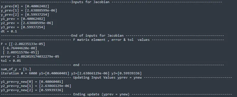
Plots :
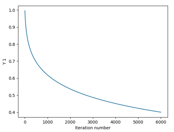
This plot shows how the value of 'Y1' changes with every iteration .
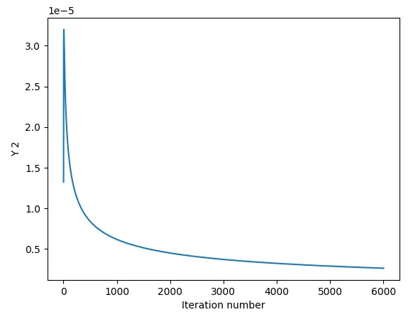
This plot shows how the value of 'Y2' changes with every iteration .
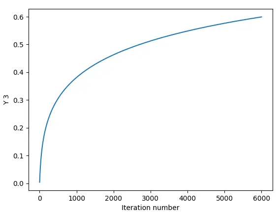
This plot shows how the value of 'Y3' changes with every iteration .
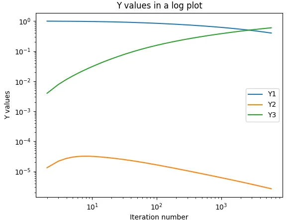
This plot shows how the value of 'Y1, Y2 ,Y3' changes with every iteration .
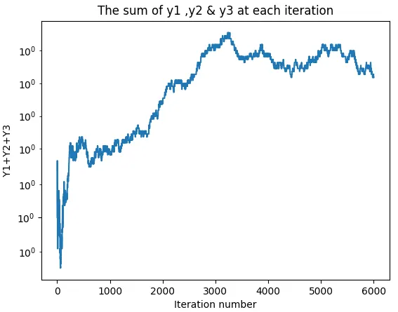
This plot shows us the sum of 'Y1 ,Y2 ,Y3' at every iteration
ie., Y1+Y2+Y3=1 in all the iterations ,the small irregulatities that we observe is because of the small variations in the values of 'Y' .
Observation :
By using dt > 4 ,the code does'nt converge .
The plots obtained satisfy the expected results .