Project 2

Aim:

To implement clustering and then to predict the price of the car from the dataset.

Code:

Dataset:

https://www.kaggle.com/fazilbtopal/auto85

Explaination:

1. Importing all libraries which might be of use further in the code is step 1.
2. Import the csv data and the file location and the code location must be in the same directory.
3. Look for the datatypes, check for 'NA' values in the dataset. If there are any irregularities fill them with random vales to render the dataset clean.
4. Convert all the object type columns into label encoded data, here a for loop is used to convert the data into manipulatable form.
5. Use standardscaler to bring all the parameters in a similar range, avoiding this step would lead to bias in the dataset result because a high valued data column can influence the results sharply.
6. The correlation matrix is plotted to view the top most contributing factors that influence the car prices.
7. A thershold value is passed and the most contributing columns are singled out, further the kmeans algorithm is run by passing the most contributing columns as the input data.
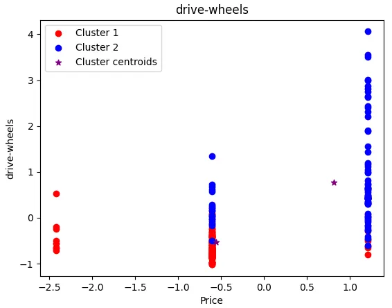
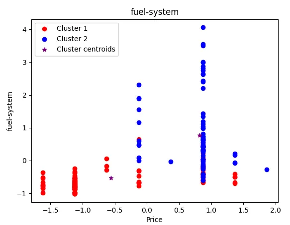
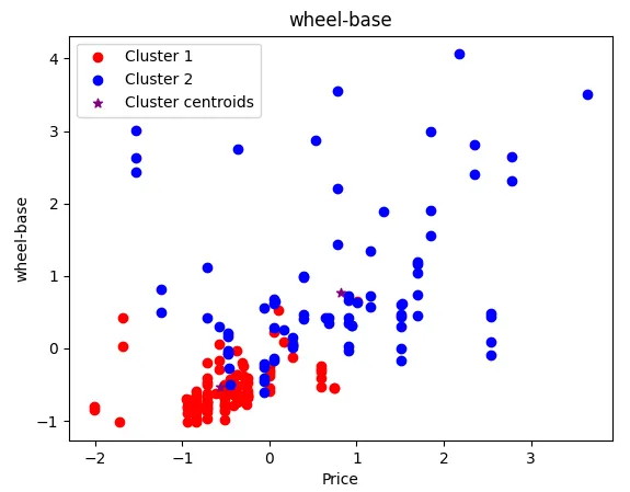
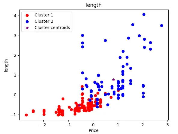
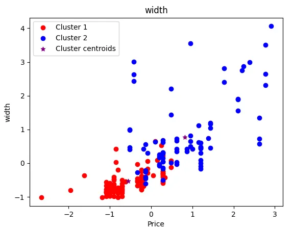
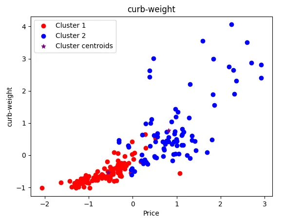
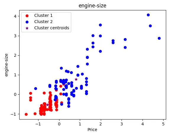
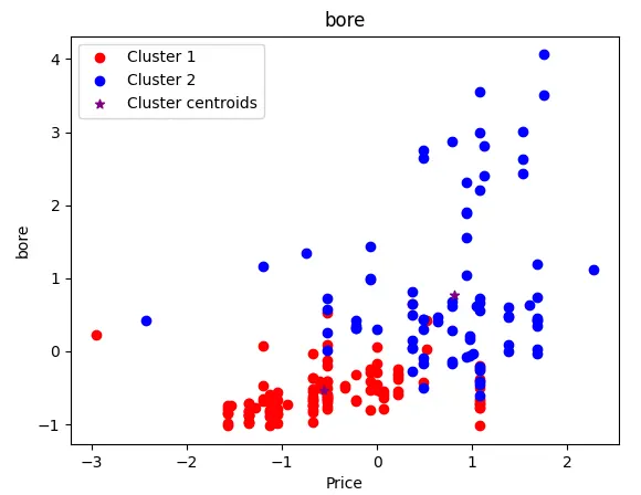
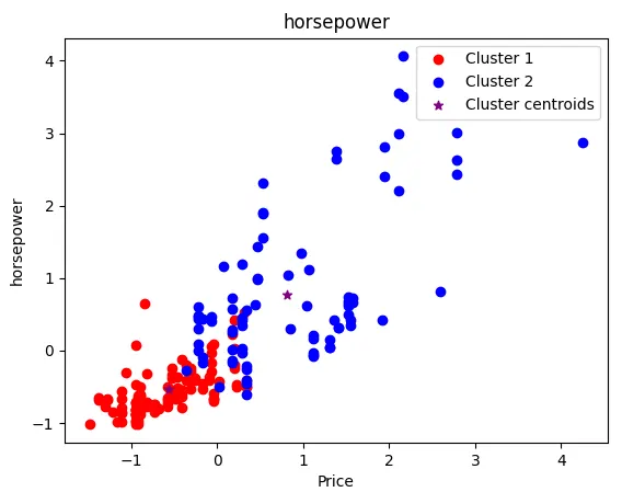
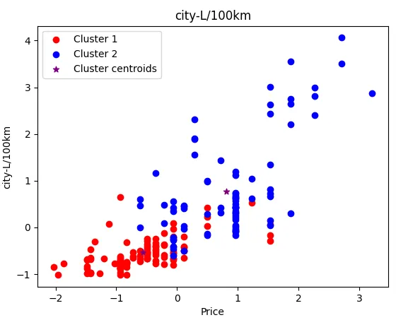
8. We isolate the clusters and plot each cluster for a particular column index against the price of the automobile.
9. Various regression algorithms are used to test the accuracy of the dataset.

import numpy as np
import pandas as pd
import matplotlib.pyplot as plt
from sklearn.preprocessing import StandardScaler
from sklearn.cluster import KMeans
import seaborn as sn

data = pd.read_csv("Auto_clean.csv")
print(data.info())
print(data.info())
print(data.count())
print(data.isnull().sum())
data['stroke'].fillna(value=np.random.randn(), inplace=True)
data['horsepower-binned'].fillna('Medium', inplace=True)
print(data.isnull().sum())

obj_df = data.select_dtypes(include=['object']).copy()
pd.set_option('display.max_rows', None)
pd.set_option('display.max_columns', None)
print(obj_df)

# method two to convert categorical data into label encoded data

name=obj_df.columns
print(type(name))

for i in range(0, len(name)):
    print(i)
    obj_df[name[i]] = obj_df[name[i]].astype('category')
    obj_df[name[i]] = obj_df[name[i]].cat.codes
    #obj_df.drop([name[i]], axis='columns', inplace=True)
    i=i+1

print(type(obj_df))
print(obj_df)
pd.set_option('display.max_columns', None)
pd.set_option('display.max_rows', None)

df = data.select_dtypes(exclude=['object'])
print(df.info())
print(df.head())

frames = [obj_df, df]
result = pd.concat(frames, axis=1)
print(result.info())

stsc=StandardScaler()
result_std=stsc.fit_transform(result)
scaled_result = pd.DataFrame(result_std, index=result.index, columns=result.columns)
pd.set_option('display.max_columns', None)
print(scaled_result.head())
print(scaled_result.describe())

corr_matrix=scaled_result.corr()
top_corr_features=corr_matrix.index
plt.figure(figsize=(12,10))
sn.heatmap(scaled_result[top_corr_features].corr(), annot=True, cmap=plt.cm.CMRmap_r)
plt.show()

threshold=0.5
a=corr_matrix['price']
res=a[a>0.5]
print(res)
res_noprice=pd.DataFrame(res.drop(['price']))
print(res_noprice)
indexed=res_noprice.index
print(indexed)


new_dat=scaled_result.loc[:, indexed]
pd.set_option('display.max_columns', None)
print(new_dat)

k_range=range(1,15)
sse=[]
for k in k_range:
    km=KMeans(n_clusters=k)
    km.fit(new_dat)
    sse.append(km.inertia_)
print(sse)
plt.plot(k_range, sse, '-*')
plt.xlabel('K value')
plt.ylabel('SSE')
plt.grid(True)
plt.title('Elbow plot (To determine best K value)')
plt.show()

km=KMeans(n_clusters=2)
print(km)
y_new=km.fit_predict(new_dat)
new_dat["Cluster_scaled"]=y_new
print(new_dat.head())

frames = [new_dat, scaled_result['price']]
new_dat = pd.concat(frames, axis=1)
print(new_dat.head())

df0=new_dat[new_dat.Cluster_scaled==0]
df1=new_dat[new_dat.Cluster_scaled==1]
"""df2=new_dat[new_dat.Cluster_scaled==2]
df3=new_dat[new_dat.Cluster_scaled==3]
df4=new_dat[new_dat.Cluster_scaled==4]"""

colname=new_dat.columns
for i in range(0,len(colname)-2):

    plt.scatter(df0[colname[i]], df0["price"],color="red",label='Cluster 1')
    plt.scatter(df1[colname[i]], df1["price"],color="blue",label='Cluster 2')
    """plt.scatter(df2[colname[i]], df2["price"],color="yellow")
    plt.scatter(df3[colname[i]], df3["price"],color="black")
    plt.scatter(df4[colname[i]], df4["price"],color="green")"""
    plt.ylabel(colname[i])
    plt.xlabel('Price')
    
    plt.title(colname[i])
    plt.scatter(km.cluster_centers_[:,0],km.cluster_centers_[:,1],color="purple",marker="*",label='Cluster centroids')
    plt.legend()
    plt.show()

from sklearn.linear_model import LinearRegression
from sklearn.model_selection import train_test_split
from sklearn.metrics import precision_score, recall_score, f1_score, accuracy_score

x=pd.DataFrame(new_dat.iloc[:, 0:10])
y=pd.DataFrame(new_dat['price'])
X_train, X_test, y_train, y_test = train_test_split(x, y, test_size=0.3, random_state=1)
clf = LinearRegression()
clf.fit(X_train,y_train)
y_pred=clf.predict(X_test)
print(y_pred)
score=clf.score(X_test,y_test)
print(score)

from sklearn.ensemble import RandomForestRegressor
regressor = RandomForestRegressor(n_estimators=20, random_state=0)
regressor.fit(X_train, y_train)
y_pred_r = regressor.predict(X_test)
print(y_pred_r)
score_r=regressor.score(X_test,y_test)
print(score_r)

from sklearn.tree import DecisionTreeRegressor
tree = DecisionTreeRegressor(max_depth=1)
tree.fit(X_train, y_train)
tree_predicted = tree.predict(X_test)
print(tree_predicted)
score_t=tree.score(X_test,y_test)
print(score_t)

print('LinearReression score = ',score)
print('RandomForestRegressor score = ',score_r)
print('DecisionTreeRegressor score = ',score_t)

Plots and results:

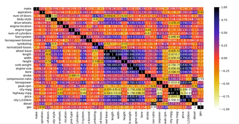
Even though the heat map looks overwhelming the above figure can be used to derive essential data that can be in our analysis.
A for loop which bings to a threshold value is used to derive the most contributing features for car price.

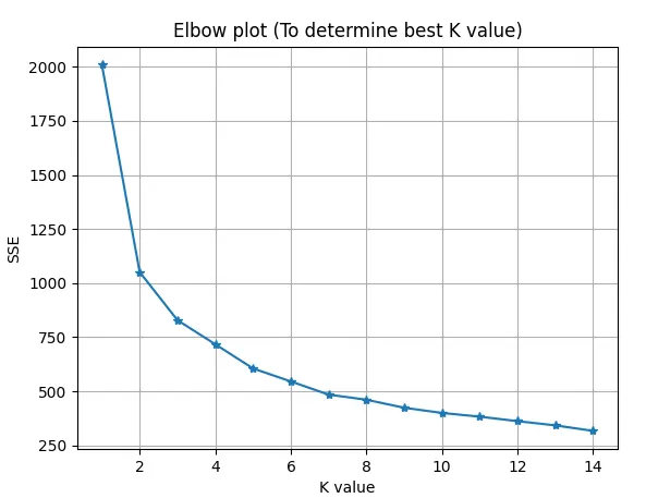
K=5 must be chosen in an ideal case but since this dataset contains so many columns it is better to use k=2 to visualise the clusters better.

Clusters:

It can be observed that as the price of the car increases the cluster group values also increase for each feature that has been plotted.
This means that as the number of features increase the cost of the car will increase.

It can be clearly seen that RandomForestRegressor produces superior score values in comparison with the other regression models.

For k=5:

import numpy as np
import pandas as pd
import matplotlib.pyplot as plt
from sklearn.preprocessing import StandardScaler
from sklearn.cluster import KMeans
import seaborn as sn

data = pd.read_csv("Auto_clean.csv")
print(data.info())
print(data.info())
print(data.count())
print(data.isnull().sum())
data['stroke'].fillna(value=np.random.randn(), inplace=True)
data['horsepower-binned'].fillna('Medium', inplace=True)
print(data.isnull().sum())

obj_df = data.select_dtypes(include=['object']).copy()
pd.set_option('display.max_rows', None)
pd.set_option('display.max_columns', None)
print(obj_df)

# method two to convert categorical data into label encoded data

name=obj_df.columns
print(type(name))

for i in range(0, len(name)):
    print(i)
    obj_df[name[i]] = obj_df[name[i]].astype('category')
    obj_df[name[i]] = obj_df[name[i]].cat.codes
    #obj_df.drop([name[i]], axis='columns', inplace=True)
    i=i+1

print(type(obj_df))
print(obj_df)
pd.set_option('display.max_columns', None)
pd.set_option('display.max_rows', None)

df = data.select_dtypes(exclude=['object'])
print(df.info())
print(df.head())

frames = [obj_df, df]
result = pd.concat(frames, axis=1)
print(result.info())

stsc=StandardScaler()
result_std=stsc.fit_transform(result)
scaled_result = pd.DataFrame(result_std, index=result.index, columns=result.columns)
pd.set_option('display.max_columns', None)
print(scaled_result.head())
print(scaled_result.describe())

corr_matrix=scaled_result.corr()
top_corr_features=corr_matrix.index
plt.figure(figsize=(12,10))
sn.heatmap(scaled_result[top_corr_features].corr(), annot=True, cmap=plt.cm.CMRmap_r)
plt.show()

threshold=0.5
a=corr_matrix['price']
res=a[a>0.5]
print(res)
res_noprice=pd.DataFrame(res.drop(['price']))
print(res_noprice)
indexed=res_noprice.index
print(indexed)


new_dat=scaled_result.loc[:, indexed]
pd.set_option('display.max_columns', None)
print(new_dat)

k_range=range(1,15)
sse=[]
for k in k_range:
    km=KMeans(n_clusters=k)
    km.fit(new_dat)
    sse.append(km.inertia_)
print(sse)
plt.plot(k_range, sse, '-*')
plt.xlabel('K value')
plt.ylabel('SSE')
plt.grid(True)
plt.title('Elbow plot (To determine best K value)')
plt.show()

km=KMeans(n_clusters=5)
print(km)
y_new=km.fit_predict(new_dat)
new_dat["Cluster_scaled"]=y_new
print(new_dat.head())

frames = [new_dat, scaled_result['price']]
new_dat = pd.concat(frames, axis=1)
print(new_dat.head())

df0=new_dat[new_dat.Cluster_scaled==0]
df1=new_dat[new_dat.Cluster_scaled==1]
df2=new_dat[new_dat.Cluster_scaled==2]
df3=new_dat[new_dat.Cluster_scaled==3]
df4=new_dat[new_dat.Cluster_scaled==4]

colname=new_dat.columns
for i in range(0,len(colname)-2):

    plt.scatter(df0[colname[i]], df0["price"],color="red",label='Cluster 1')
    plt.scatter(df1[colname[i]], df1["price"],color="blue",label='Cluster 2')
    plt.scatter(df2[colname[i]], df2["price"],color="orange",label='Cluster 3')
    plt.scatter(df3[colname[i]], df3["price"],color="black",label='Cluster 4')
    plt.scatter(df4[colname[i]], df4["price"],color="green",label='Cluster 5')
    plt.ylabel(colname[i])
    plt.xlabel('Price')
    
    plt.title(colname[i])
    plt.scatter(km.cluster_centers_[:,0],km.cluster_centers_[:,1],color="purple",marker="*",label='Cluster centroids')
    plt.legend()
    plt.show()

from sklearn.linear_model import LinearRegression
from sklearn.model_selection import train_test_split
from sklearn.metrics import precision_score, recall_score, f1_score, accuracy_score

x=pd.DataFrame(new_dat.iloc[:, 0:10])
y=pd.DataFrame(new_dat['price'])
X_train, X_test, y_train, y_test = train_test_split(x, y, test_size=0.3, random_state=1)
clf = LinearRegression()
clf.fit(X_train,y_train)
y_pred=clf.predict(X_test)
print(y_pred)
score=clf.score(X_test,y_test)
print(score)

from sklearn.ensemble import RandomForestRegressor
regressor = RandomForestRegressor(n_estimators=20, random_state=0)
regressor.fit(X_train, y_train)
y_pred_r = regressor.predict(X_test)
print(y_pred_r)
score_r=regressor.score(X_test,y_test)
print(score_r)


from sklearn.tree import DecisionTreeRegressor
tree = DecisionTreeRegressor(max_depth=1)
tree.fit(X_train, y_train)
tree_predicted = tree.predict(X_test)
print(tree_predicted)
score_t=tree.score(X_test,y_test)
print(score_t)

print('LinearReression score = ',score)
print('RandomForestRegressor score = ',score_r)
print('DecisionTreeRegressor score = ',score_t)

Plots:

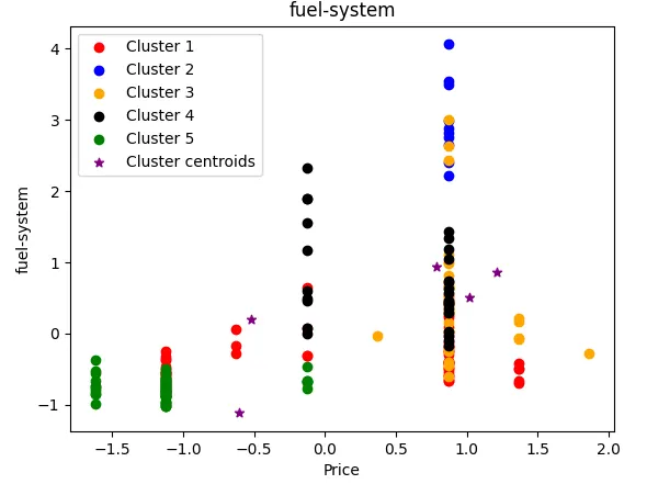
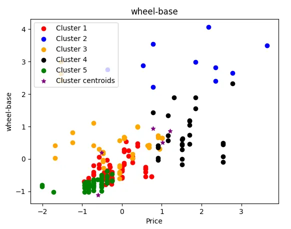
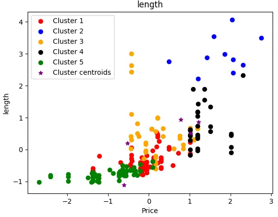
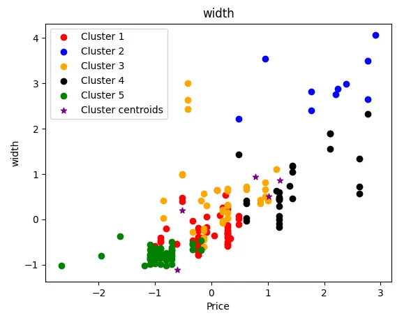
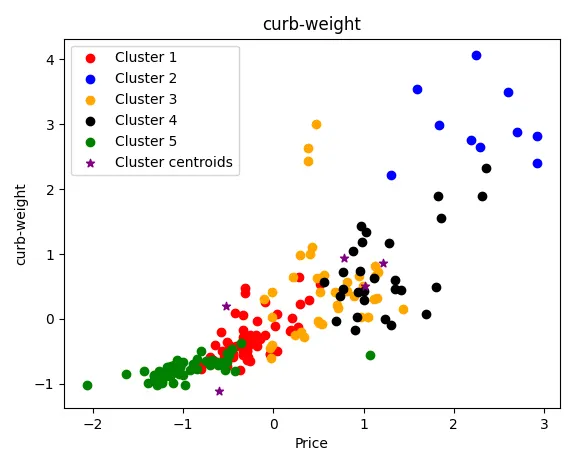
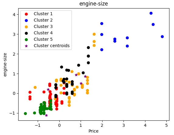
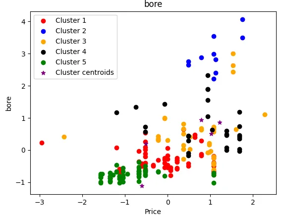
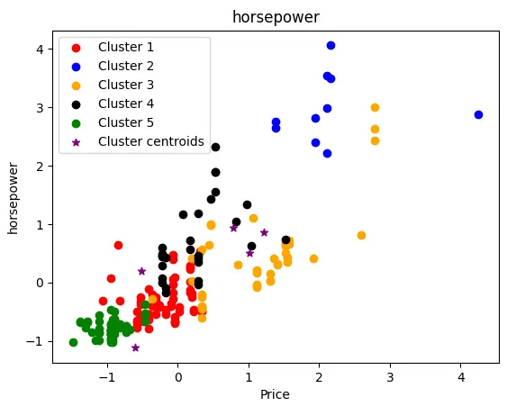
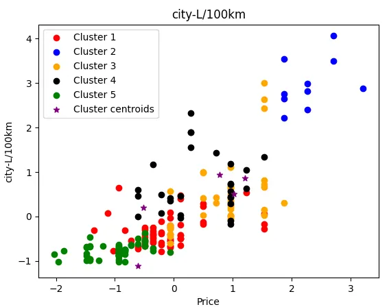
From the below scatter plots it can be clearly observed how the clusters look so chaotic, hence it's better to use k=2 to visualise the data better

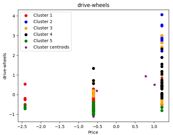
Here there are a lot of green clusters in the mid range with respect to the frive-wheel feature.

References:

https://stackabuse.com/random-forest-algorithm-with-python-and-scikit-learn/

https://inria.github.io/scikit-learn-mooc/python_scripts/trees_regression.html