Week 8 - Simulating Cyclone separator with Discrete Phase Modelling
Aim:- To perform analysis on cyclone separator and calculate the separation efficiency and pressure drop.
Objective:-
- To write a few words about any four empirical models used to calculate the cyclone separator efficiency.
- To perform an analysis on a given cyclone separator model by varying the particle diameter from 1 μm to 5 μm and calculate the separation efficiency in each case. Discuss the results. [Use both the velocity's as 3m/sec.]
- To perform an analysis on a given cyclone separator model by varying the particle velocity from 1 m/sec to 5 m/sec and calculate the separation efficiency and pressure drop in each case. Discuss the results. [Use particle diameter size as 5 μm for all cases & keep flow velocity same as particle velocity]
Note:
Boundary Conditions:-
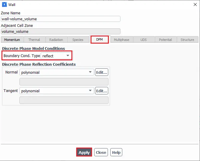
Inlet and wall:- Reflect
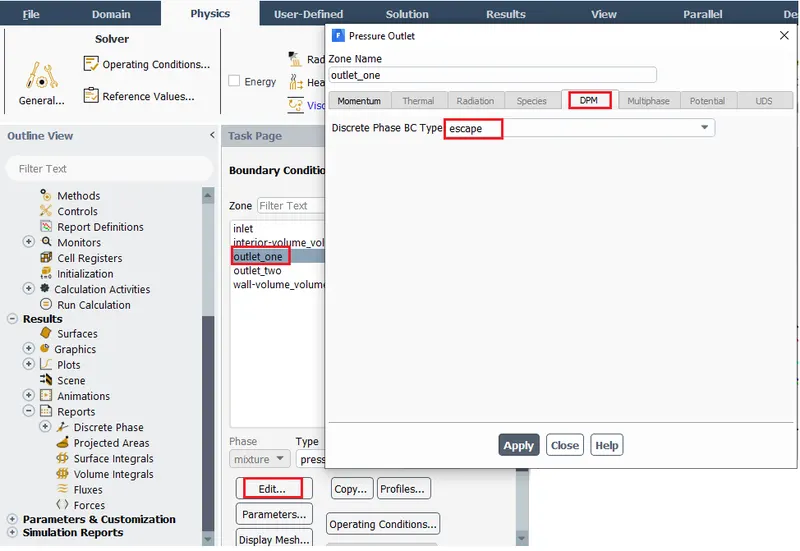
Outlet(Top):- Escape
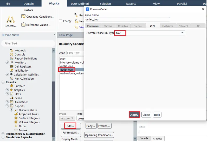
Outlet(Bottom/dustbin) - Trap
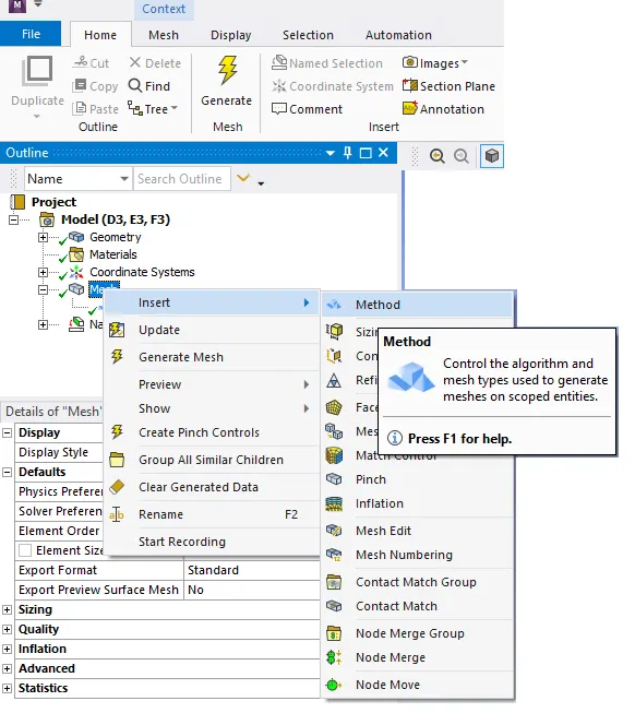
Structural mesh gives the best results, so you can use cutcell meshing approach available in Ansys Meshing.
FORMULA:
Seperation effeciency:
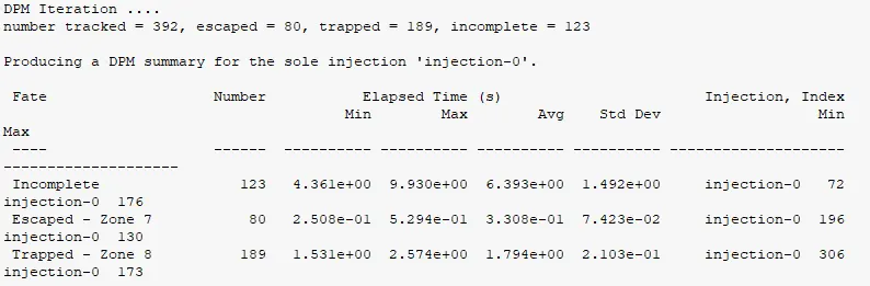
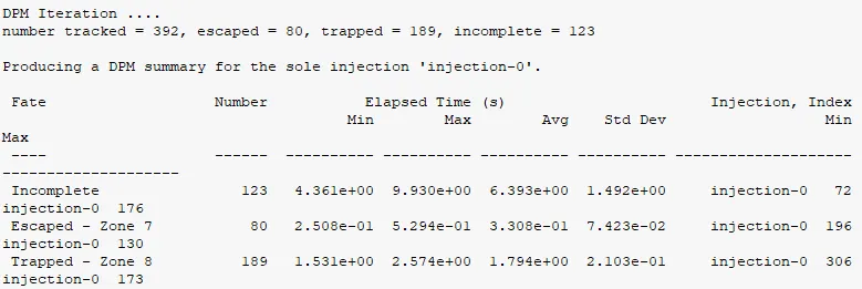
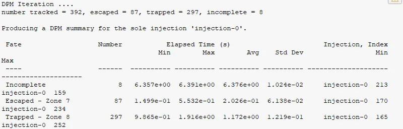
`eta=[trapped]/[tracked]*100`
Pressure drop:
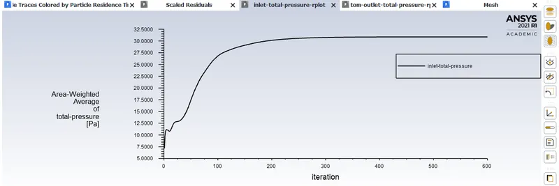
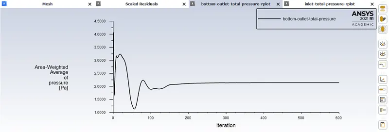
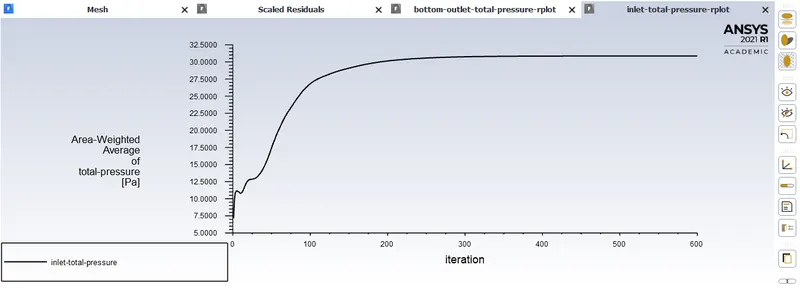
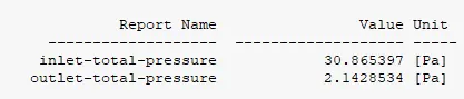
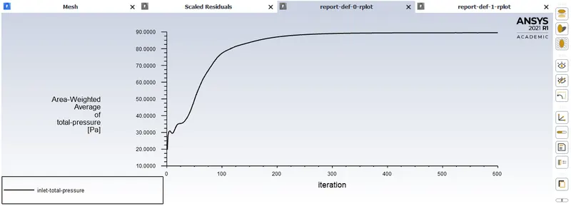
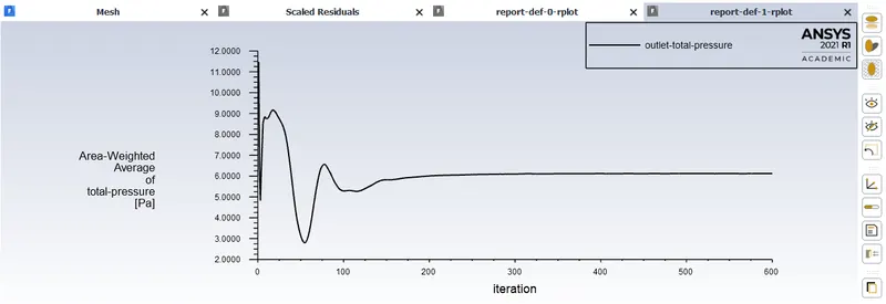
Pressure drop = Total pressure at inlet - Total pressure at outlet (bottom outlet)
Cyclone seperator:
- Cyclones are devices that employ a centrifugal force generated by a spinning gas stream to separate particles from the carrier gas.
- Their simple design, low maintenance costs and adaptability to a wide range of operating conditions such as sizes and flow rates make cyclones one of the most widely used particle removal devices.
- By using suitable materials and methods of construction, cyclones may be adapted for use in extreme operating conditions: high temperature, high pressure, and corrosive gases.
- Cyclones are important particle removal devices in both engineering and process operations.
An inaccuracy in cyclone efficiency prediction may result in an inefficient design of cyclone separators.
Models to predict the behaviour of cyclones are usually empirical.
It remains largely a process of trial and error, since empirical cyclones models are only applicable to specific cyclone geometries.
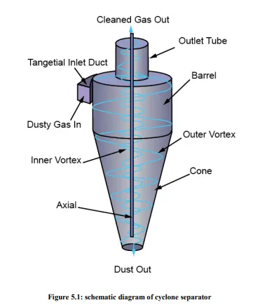
The four different cyclone efficiency empirical models are namely:
- IOZIA AND LEITH MODEL
- LI AND WANG MODEL
- KOCH AND LICHT MODEL
- LAPPLE MODEL
1. IOZIAAND LEITH MODEL
Iozia and Leith (1990) logistic model is a modified version of Barth (1956) model which is developed based on force balance. The model assumes that a particle carried by the vortex endures the influence of two forces: a centrifugal force, Z, and a flow resistance, W. Core length, `z_c`, and core diameter, `d_c`, are given as
`z_c = (H - S) - [(H - S)/((D/B) -1)] [(dc / B) -1]` for `d_c > B`
`z_c = H - S` for `d_c < B`
`d_c= 0.47((ab)/D^2)^-0.25 (D_e/D)^1.4`
The addition made by Iozia and Leith on the original Barth (1956) model are the core length `z_c` and slope parameter `beta` expression which is derived based on the statistical analysis of experimental data of cyclone with D = 0.25 m. The collection efficiency `eta_i` of particle diameter `d_(p i)` can be calculated from
`eta_i = 1/(1+(d_(pc) / overline d_(p i))^(beta)`
where `d_(pc)` is the 50% cut size given by Barth (1956)
`d_(pc) = [(9muQ)/(pi p_p z_c v_(tmax)^(2))]^0.5`
2. LI AND WANG MODEL
The Li and Wang (1989) model includes particle bounce or re-entrainment and turbulent diffusion at the cyclone wall. A two-dimensional analytical expression of particle distribution in the cyclone is obtained. Li and Wang model was developed based on the following assumptions:
• The radial particle velocity and the radial concentration profile are not constant, for uncollected particles within the cyclones.
• Boundary conditions with the consideration of turbulent diffusion coefficient and particle bounce re-entrainment on the cyclone wall are:
`c = c_0` at `theta = 0`
`D_r ((delc)/(delr))= (1- alpha)wc` at `r = D/2`
The tangential velocity is related to the radius of cyclone by:
`uR^n` = constant.
The concentration distribution in a cyclone is given as:
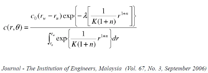
where
`k = ((1-n)(rho_p-rho_g)d^2Q)/(18mub(r_w^(1-n) - r_n^(1-n)))`
and
`lambda =((1-alpha)kw_w)/(D_r r_w^n)`
The resultant expression of the collection efficiency for particle of my size is given as
`eta_i = 1 - exp {-lambda theta_1}`
where
`theta_1 = 2pi (S + L) / a`
3. KOCH AND LICHT MODEL
Koch and Licht (1977) collection theory recognized the inherently turbulent nature of cyclones and the distribution of gas residence times within the cyclone. Koch and Licht describe particle motion in the entry and collection regions with the additional following assumptions:
• The tangential velocity of a particle is equal to the tangential velocity of the gas flow, i.e. there is no slip in the tangential direction between the particle and the gas.
• The tangential velocity is related to the radius of cyclone by:
`uR^n` = constant.
A force balance and an equation on the particles collection yields the grade efficiency `eta_i`
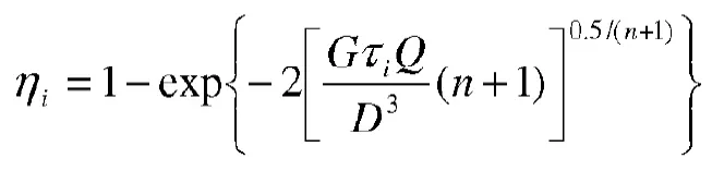 .
.
where
`G = (8k_c)/(k_a^2 k_b^2`
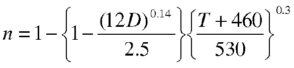
`tau_i = (rho_p d_(p i) ^2) /(18 mu)`
G is a factor related to the configuration of the cyclone, n is related to the vortex and `tau` is the relaxation term.
4. LAPPLE MODEL
Lapple (1951) model was developed based on force balance without considering the flow resistance. Lapple assumed that a particle entering the cyclone is evenly distributed across the inlet opening. The particle that travels from inlet half width to the wall in the cyclone is collected with 50% efficiency. The semi empirical relationship developed by Lapple (1951) to calculate a 50% cut diameter, `d_(pc)`, is
`d_(pc) = [(9mub)/(2piN_ev_i(rho_p-rho_g))]^(1/2)`
where `N_e` is the number of revolutions
`N_e = 1/a[h + (H - h)/ 2]`
The efficiency of collection of any size of particle is given by
`eta_i = 1/(1 + (d_(pc) / (overline(d_(p i))))^2`
RNG Model:
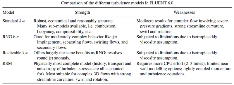
The standard k-`epsi`, RNG k-`epsi` and Realizable k-`epsi` models were not optimized for the strongly swirling flows typically found in cyclones. Turbulence may be stabilized or destabilized in the parts of flow domain where strong streamline curvature is present. However, to reduce the computational effort, the RNG k-`epsi` model can be used with about 12% deviation on experimental data.
RNG k-`epsi` model underestimates the variation of the axial velocity profile across the radial direction and also overestimates the magnitude of the tangential velocity and the cyclone pressure 100 drop. The Reynolds stress model requires the solution of transport equations for each of the Reynolds stress components as well as for dissipation transport without the necessity to calculate an isotropic turbulent viscosity field. The Reynolds Stress turbulence model yields an accurate prediction of swirl flow pattern, axial velocity, tangential velocity and pressure drop on cyclone simulations.
Mesh:
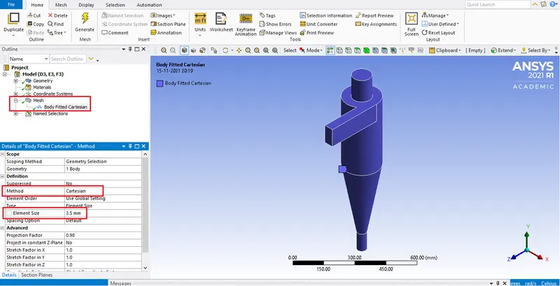
Hit on generate mesh.
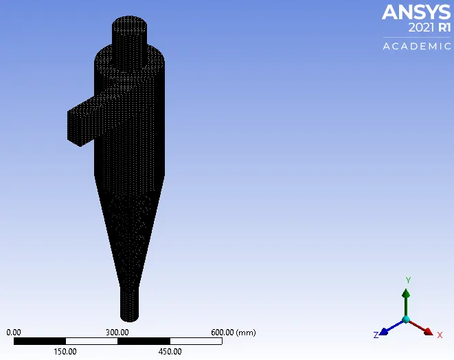
Unsuccessful meshing:
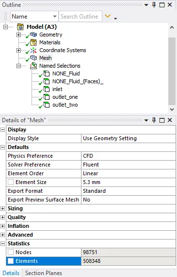
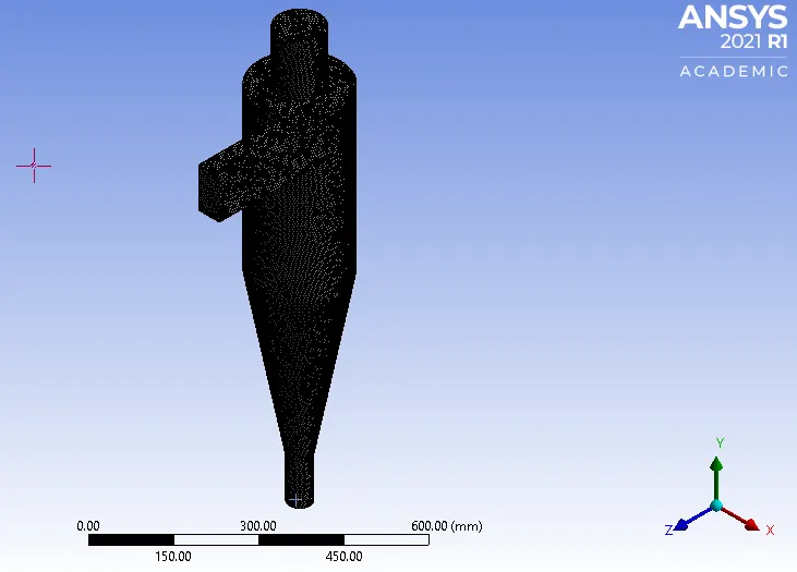
This leads to errors.
Setup:
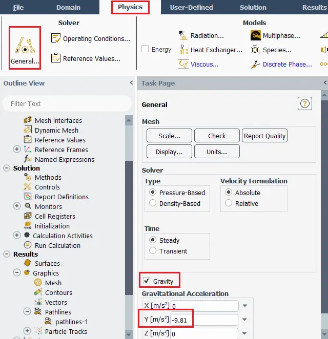
- First to add acceleration due to gravity, the gravity must be checked.
The acceleration due to gravity of -9.81m/s must be entered. - Viscous model:
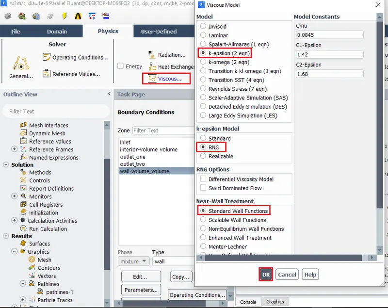
Physics > Under models: Viscous model > `k-epsi` model > under `k-epsi` RNG > Near wall treatment: Standard wall function > OK - Discrete phase model:
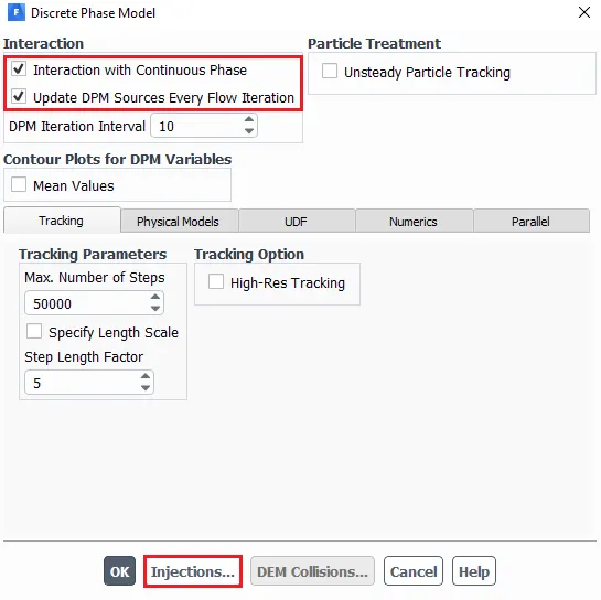
Check the 2 boxes
a) Interactions with continous phase: Gives us a chance to calculate source terms at every iteration
b) Update DPM sources every few iterations.
DPM update interval = 10: Update DPM Sources Every Flow Iteration allows you to control how DPM sources are applied to the continuous phase equations. When this option is enabled, the sources are successively updated in the flow equations at every flow solver iteration.
(refer: https://ansyshelp.ansys.com/account/secured?returnurl=/Views/Secured/corp/v211/en/flu_ug/flu_ug_sec_pt_interaction.html?q=DPM%20iteration%20interval)
Tracking: Gives the number of time steps & it is used to compute the single particle trajectory. In case Ansys Fluent exceeds this number of steps, it will automatically cancel the reporting of trajectory.
This will happen when the particle is trapped in the recirculation region.
Injections:
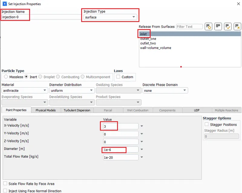
To specify the injections in the discrete particles onto the continous phase.
Injections(Under DPM options) > Create > Particle type: Inert > Materials: Anthracite > Injection type: Surface injections > Release from: Inlet > Variable: X velocity = 3m/s (for case 1) or 1m/s (for case 2) > Diameter: (1 to 5)`mum` for case 1 & `mum`for case 2 > Total flow rate: 1e-20 > OK > Close. - Boundary conditions:
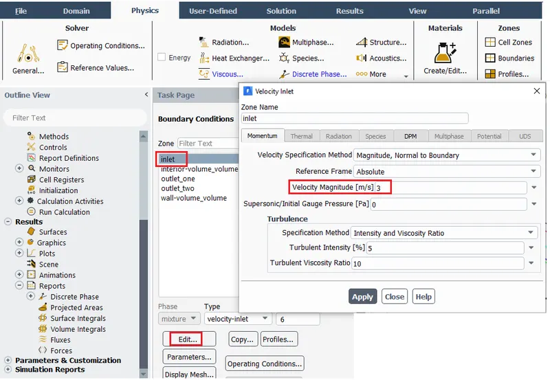
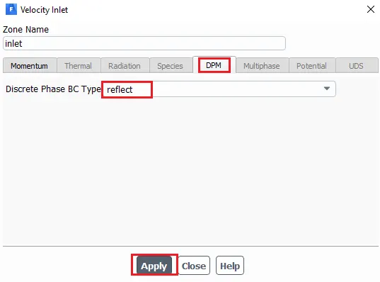
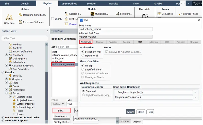
Under 'Physics' > click the appropriate zone to set the DPM condition > Hit 'Edit'.
For inlet & wall: Reflect & under 'momentum' change inlet velocity magnitude to 3m/s.
For Outlet(top): Escape.
For Outlet(Bottom/dustbin): Trap. - Solution:
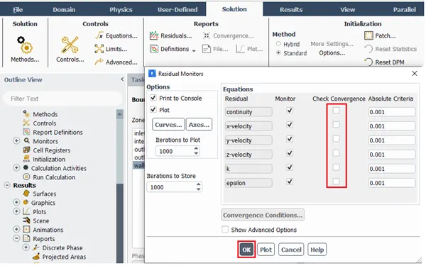
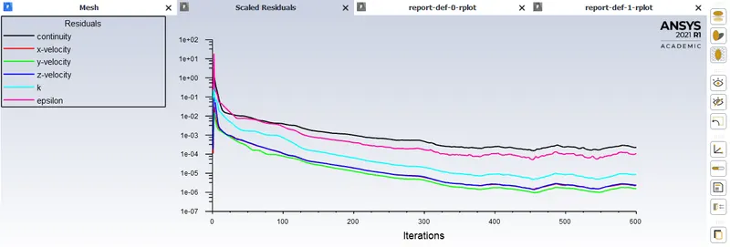
Under 'reports' > 'Residuals' > Uncheck the 'Check convergence box'.
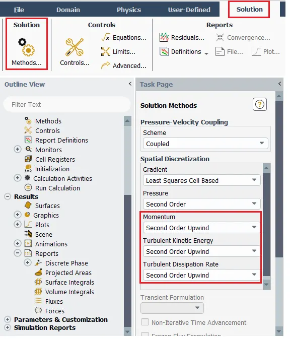
Under 'solution' hit 'Method' > Change 'Turbulent kinetic energy' and 'Turbulent dissipation rate' to Second order upwind scheme
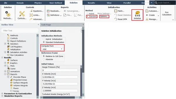
Choose standard initialization: Hit 'Options' > Compute from 'inlet'.
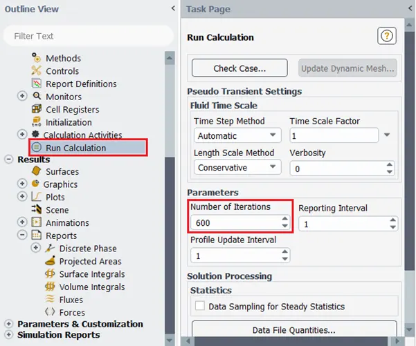
Hit on 'run calculation'
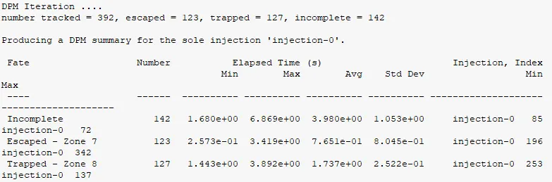
Number of iterations: 600 > 'Run calculation' - Note the values displayed in console:
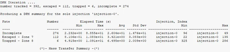
If the values for tracked, escaped ,trapped & incomplete are not visible.
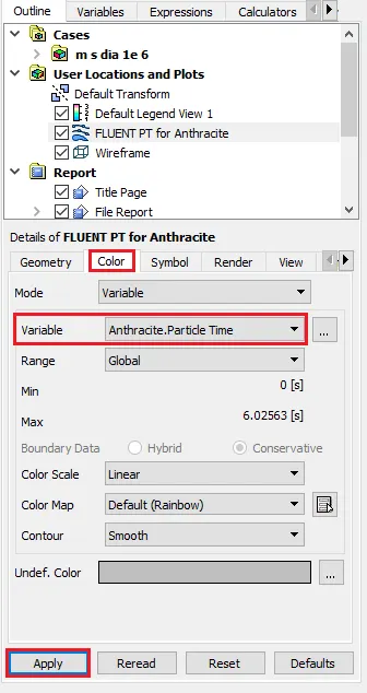
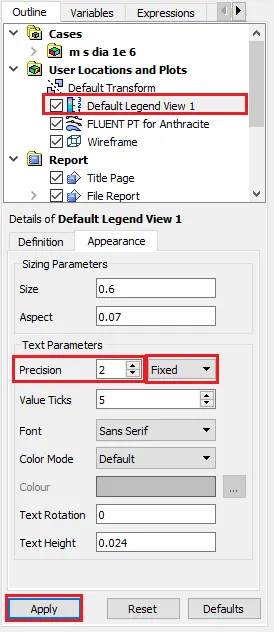
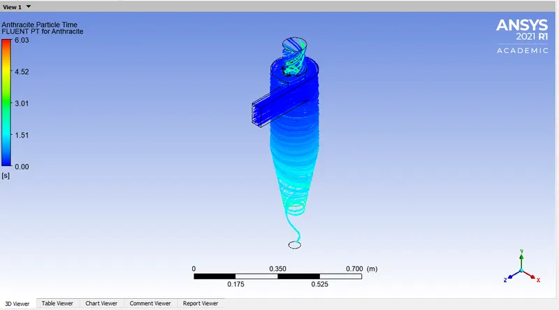
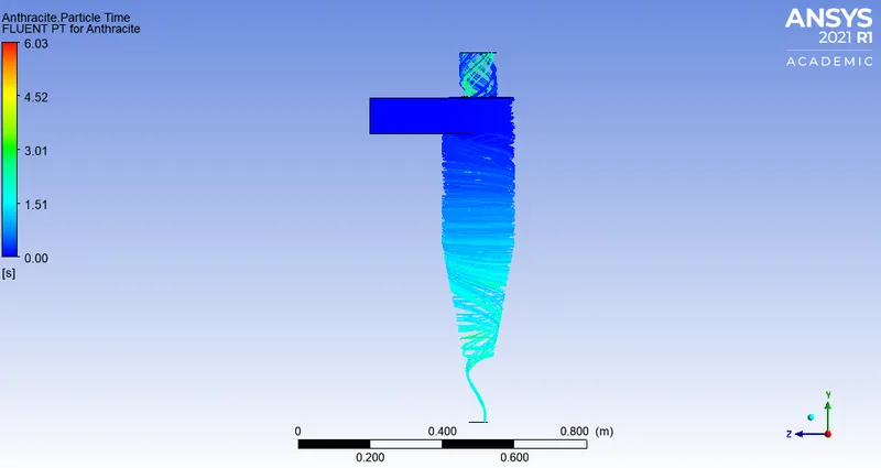
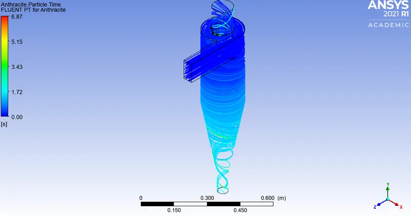
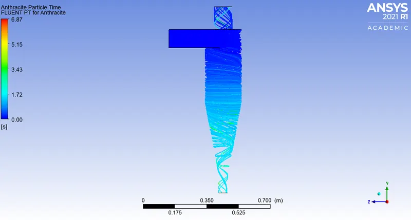
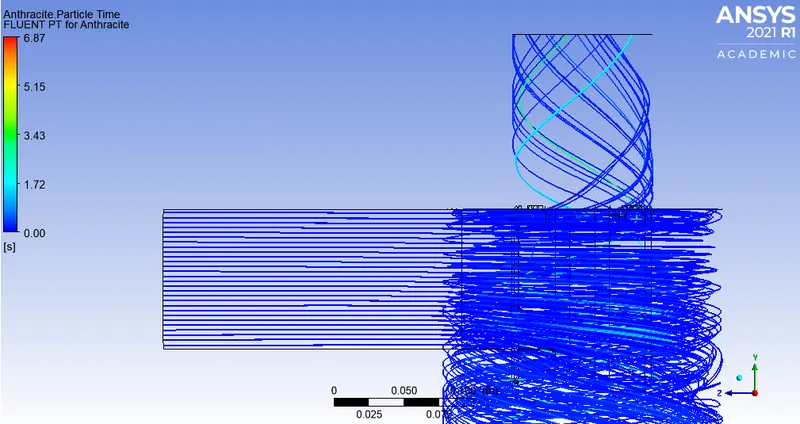
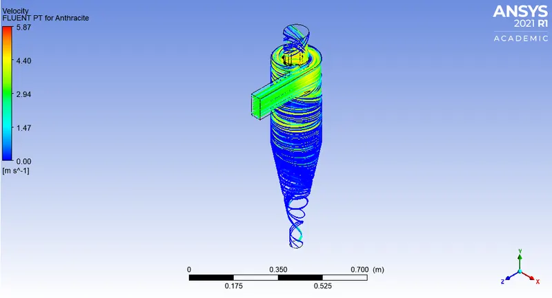
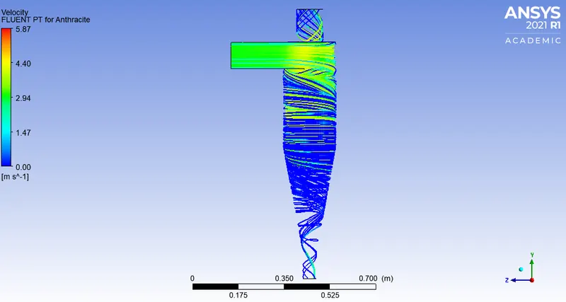
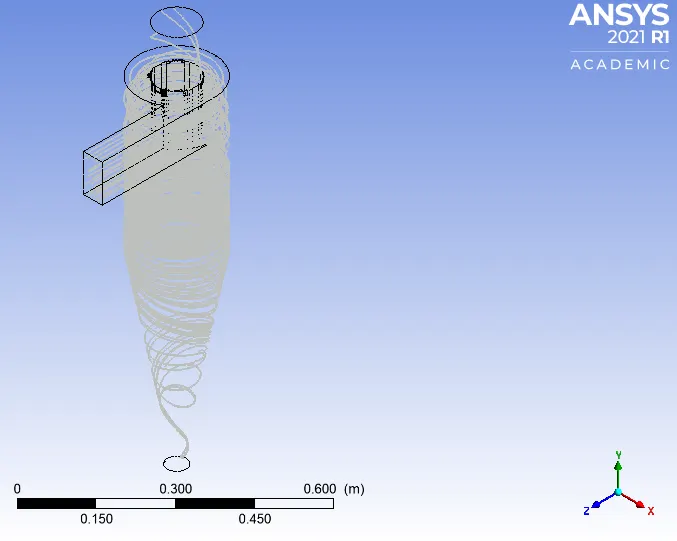
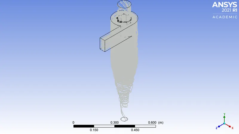
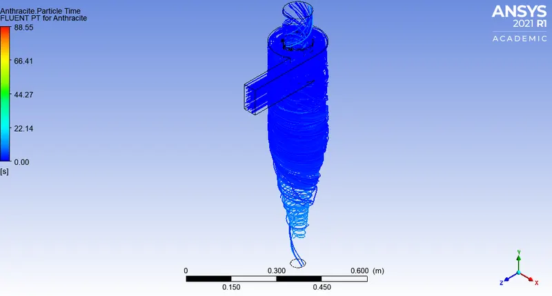
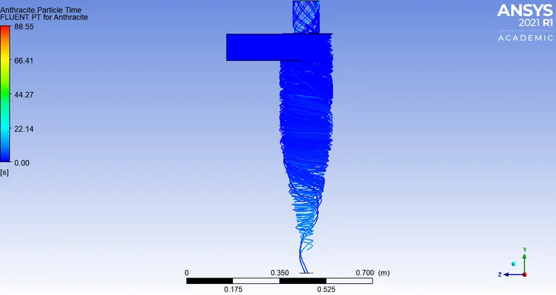
Under 'outline' > Under 'results' > Double click on 'graphics' > In the task page, double click 'particle track' under 'graphics' > Report type 'summary' > Colour by 'particle residence time' > Relese from injections: Select 'Injection' > Save and display.
Now the particle trecking data is visible. - Total pressure: Report creation
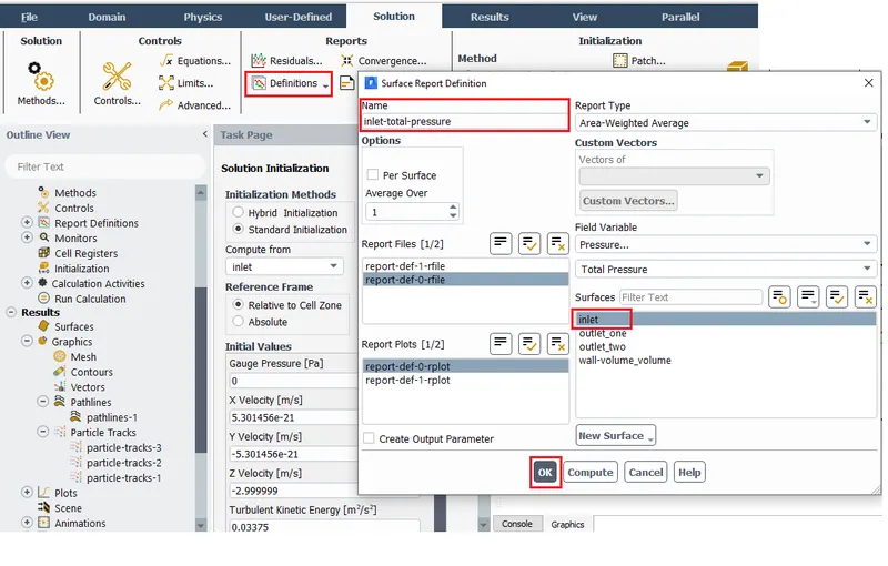
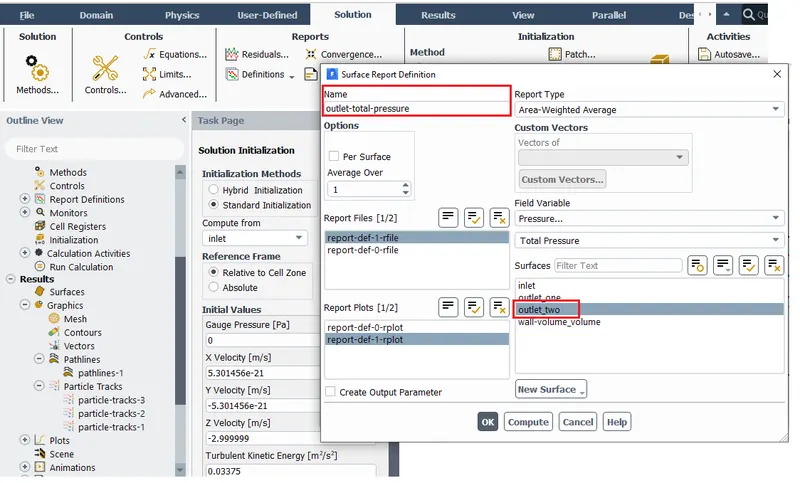
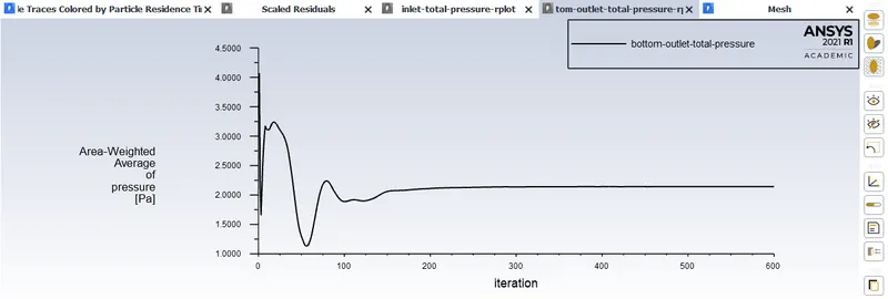
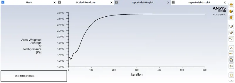
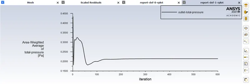
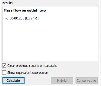
Solution > Under reports: Definition > Surface definition > Area weighted average > Field variable: Total pressure > Surfaces: Inlet or Outlet_two (bottom outlet) > Check 'Report file' & 'Report plot' > Ok - Extracting particle tracking data:
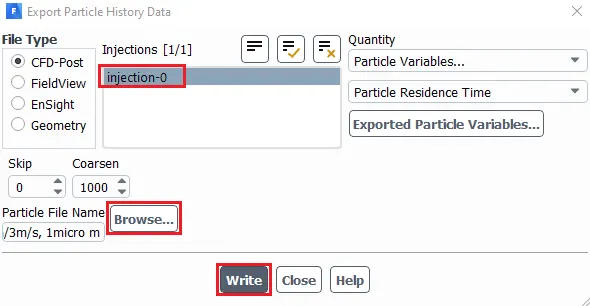
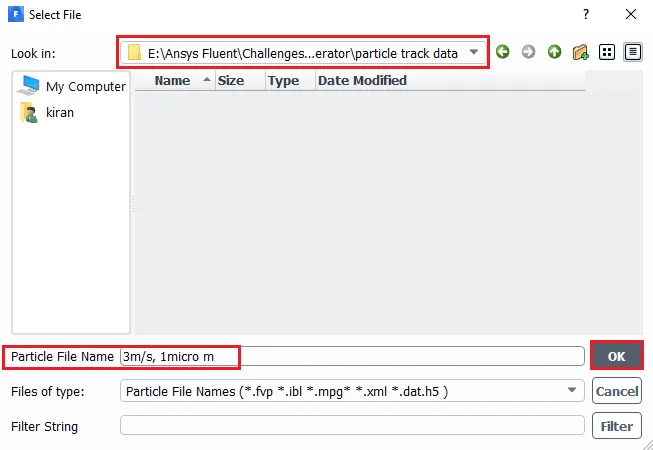
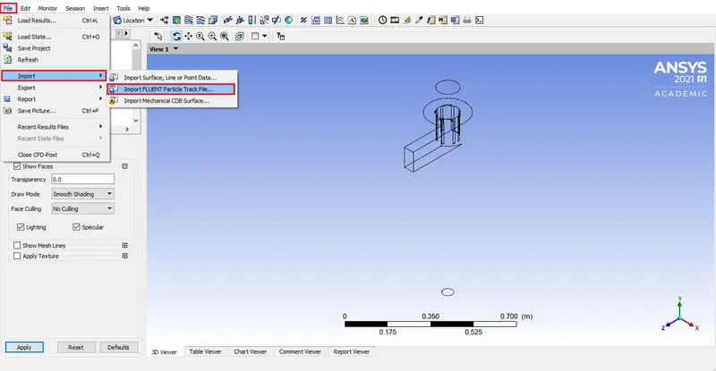
File > Export > Particle history data > Quantity: 'Particle variables' & 'Particle residence time' > Select 'Injections' Under Injections > Browse and select the appropriate location > Write
Pictoral step by step process:
DPM setup:
Boundary conditions:
Inlet:
Outlet(top):
Outlet(bottom):
Wall:
Solution:
Pressure:
Exporting particle history data:
Plots:
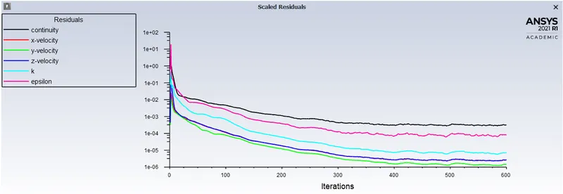
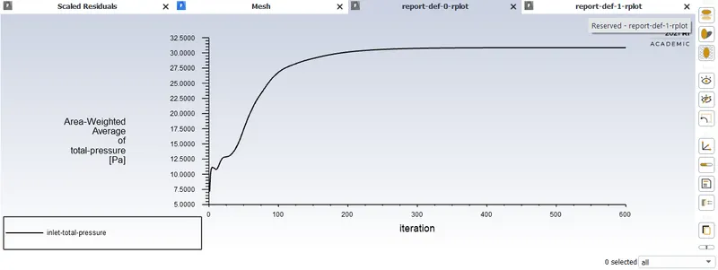
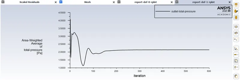
Console:
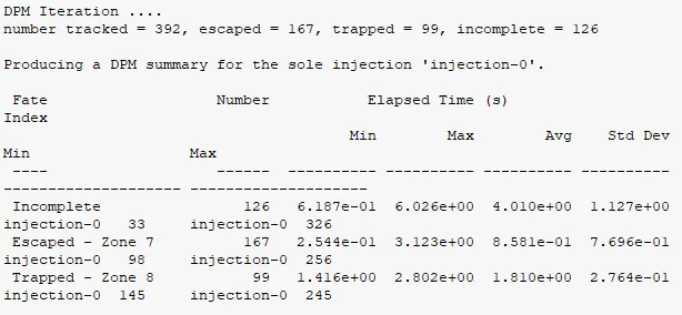
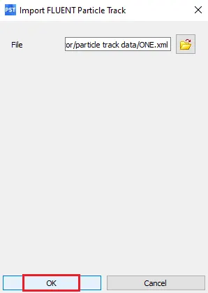
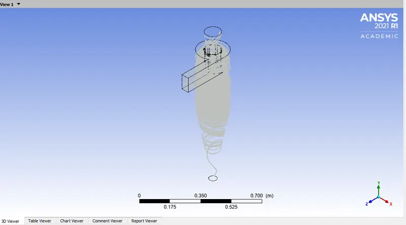
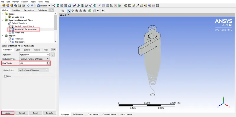
Results/CFD Post:
Results:
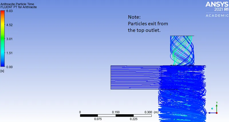
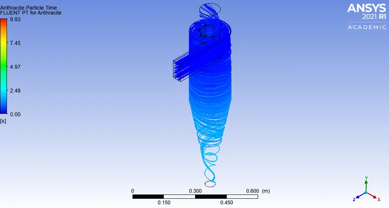
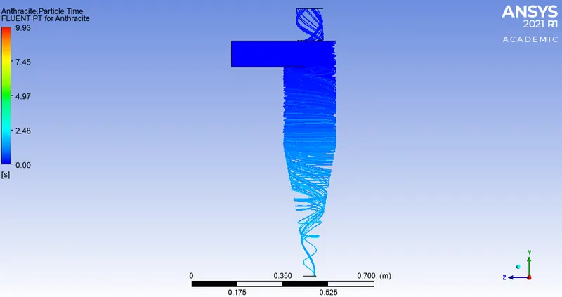
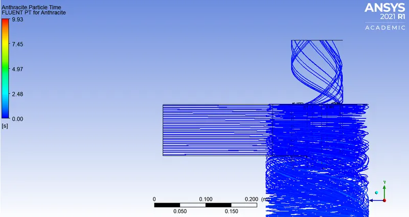
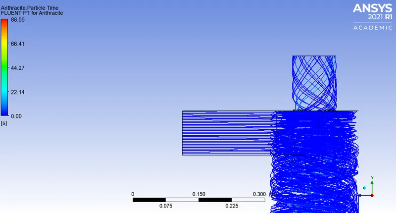
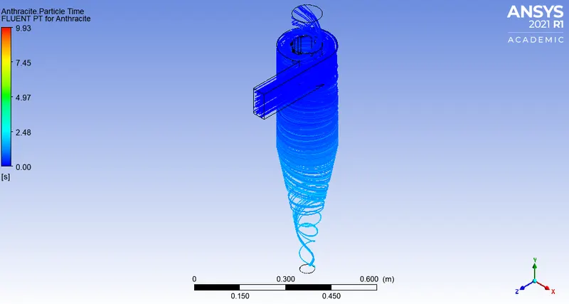
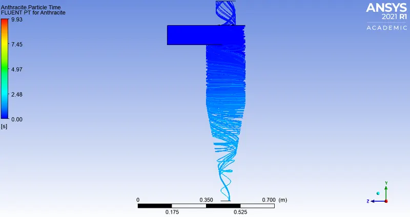
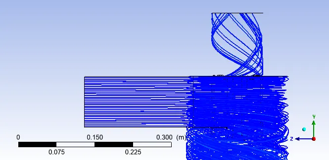
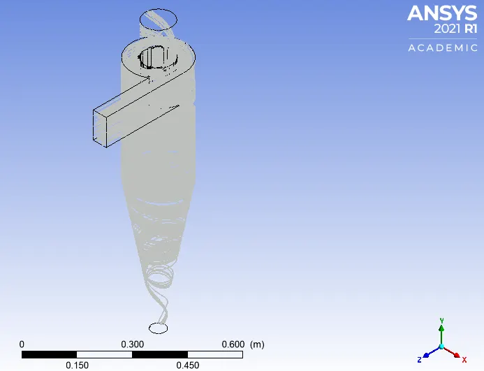
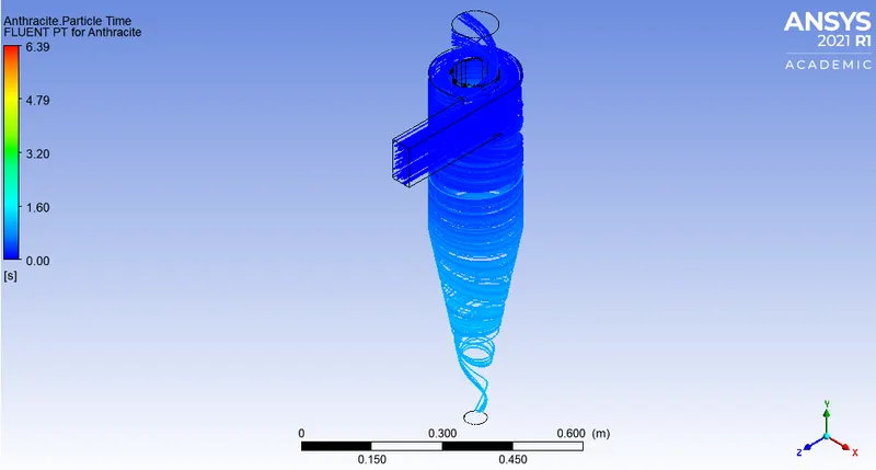
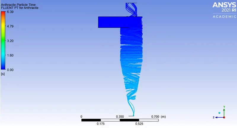
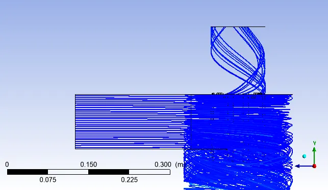
Particle Time: Shows particle residence time of each particle.
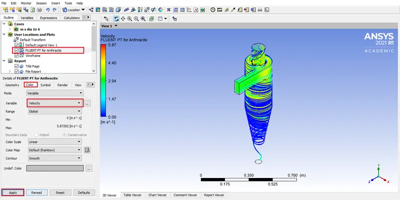
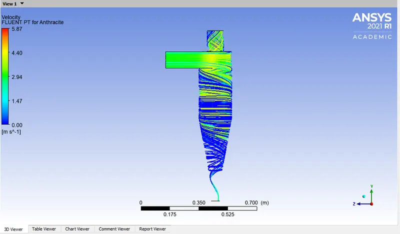
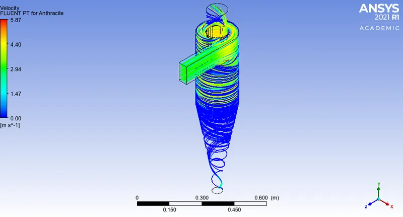
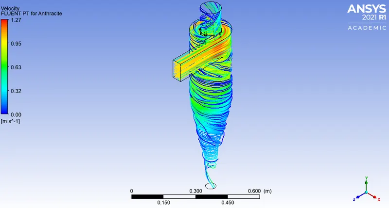
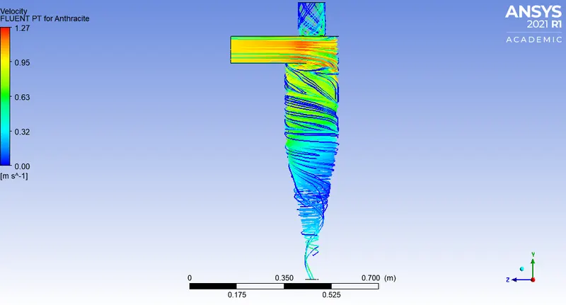
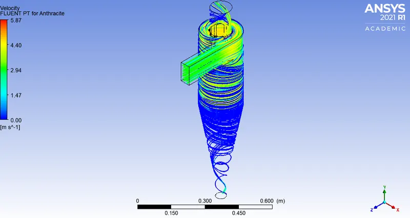
Velocity:
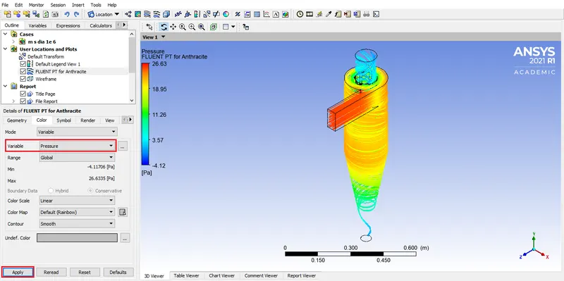
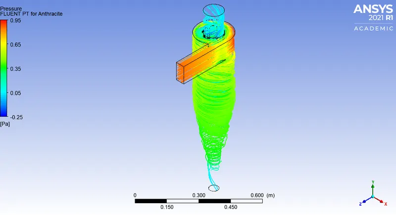
Pressure:
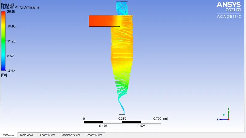
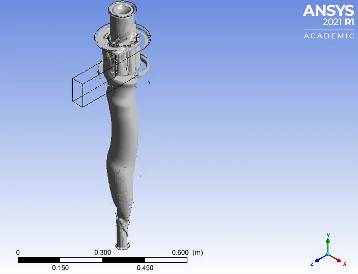
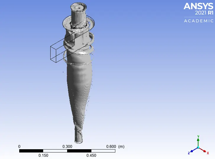
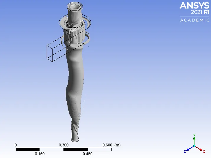
Swirling vortex:
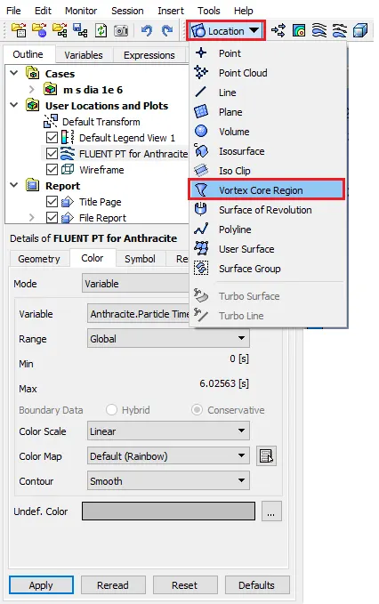
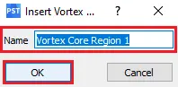
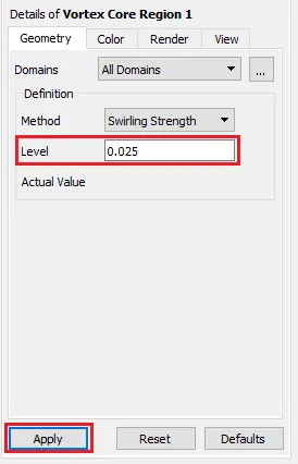
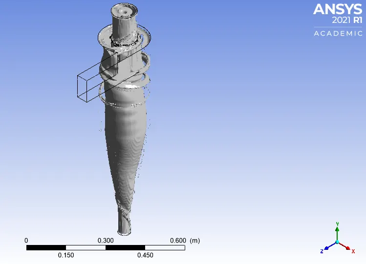
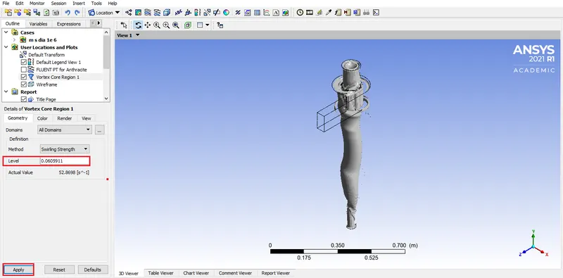
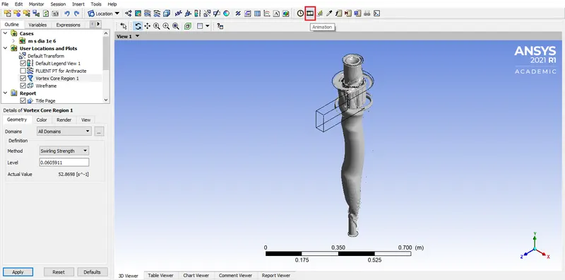
To visualise vortex generated: Video
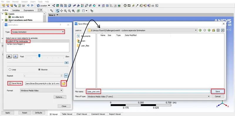
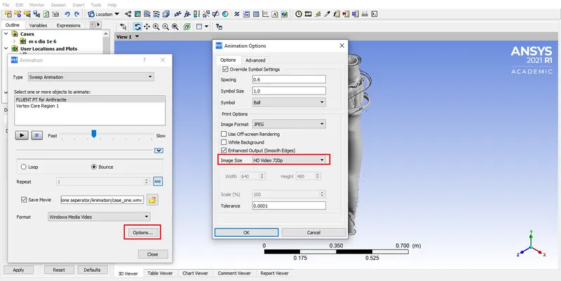
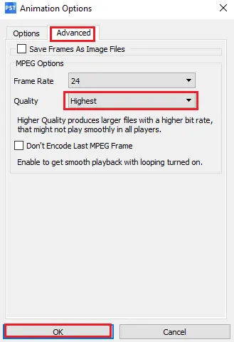
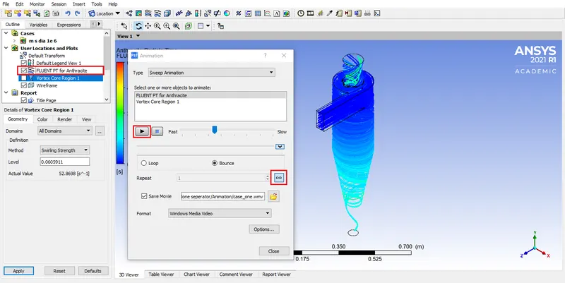
Animation: https://youtu.be/qVSuPW72cpM
More details:
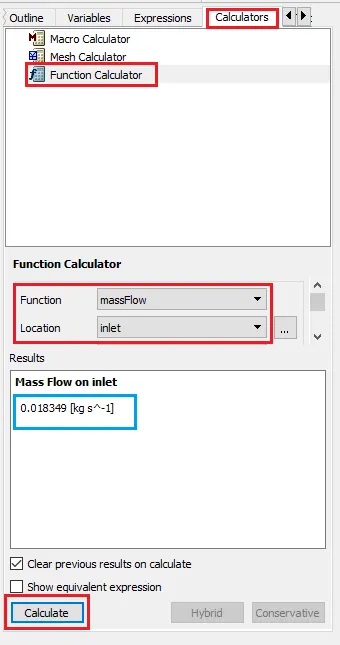
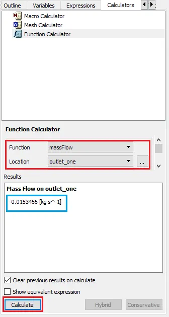
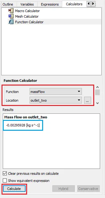
3m/s, D=3 micro meters
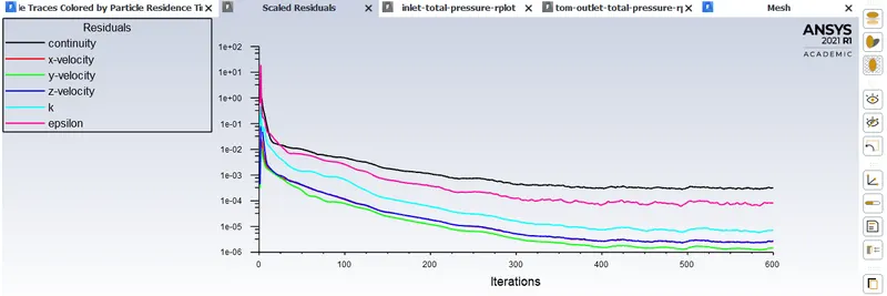
Residuals:
Plots:

Console:
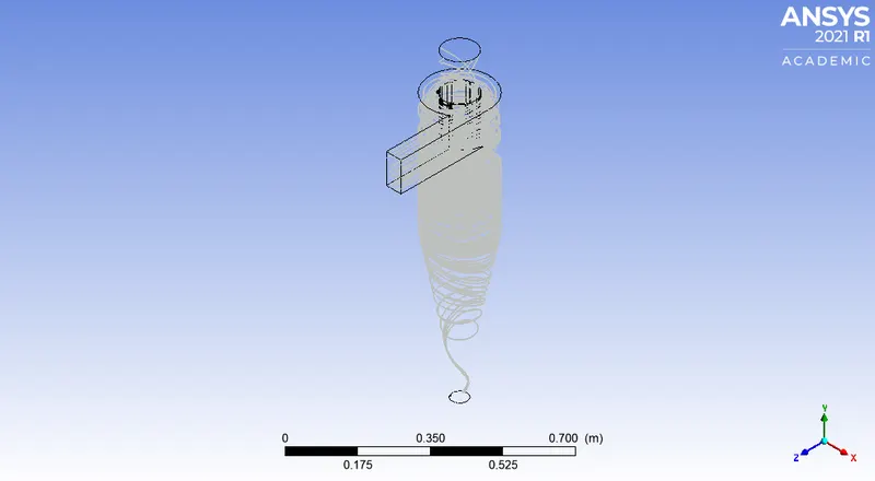
CFD Post:
Particle time:
Velocity:
Pressure:
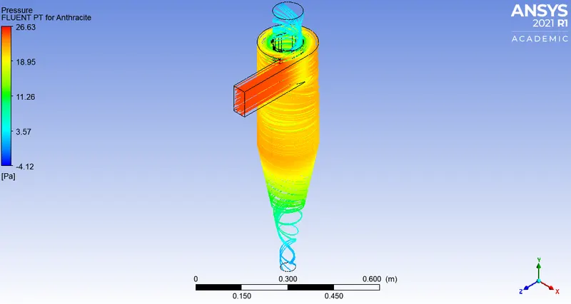
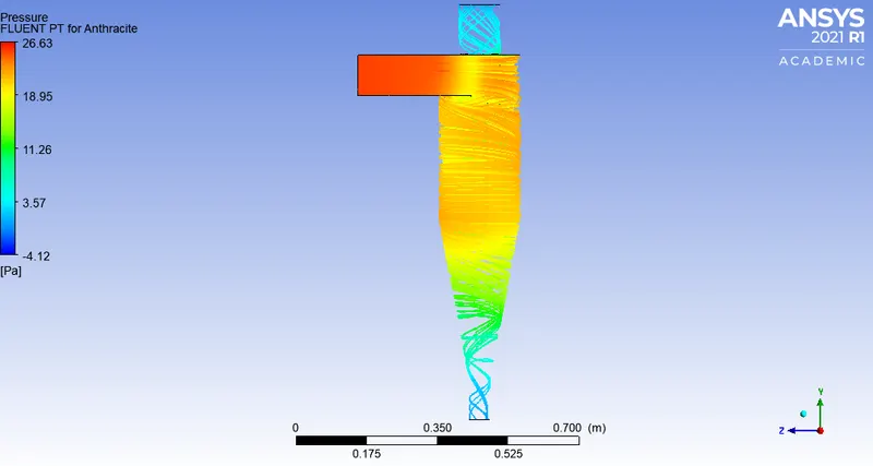
Swirling vortex:
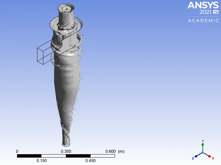
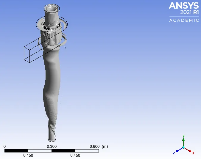
Animation: Video
Additional details:
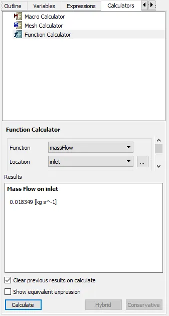
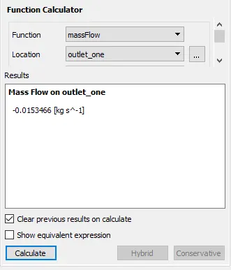
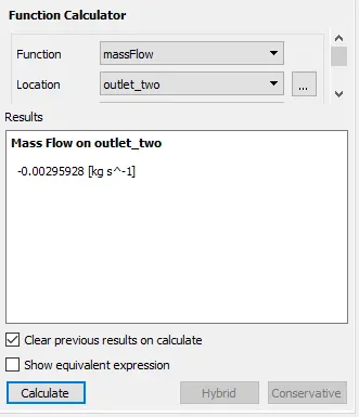
3m/s, D=5 micro meters:
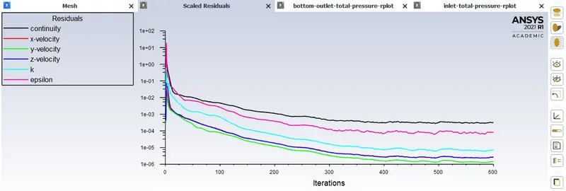
Residual:
Plots:
Console:

CFD Post:
Particle time:
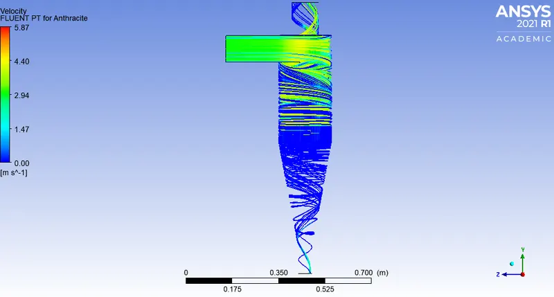
Velocity:
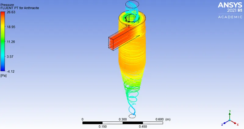
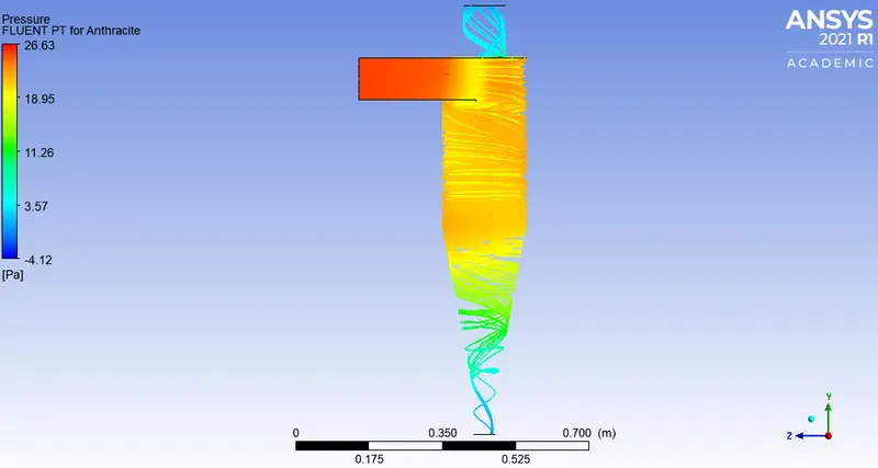
Pressure:
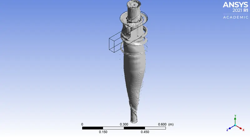
Vortex:
Animation: Video
Additional details:
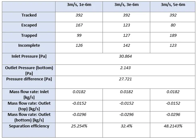
Tabulated results: Case 1
Case 2:
1m/s, 5 micro meters:
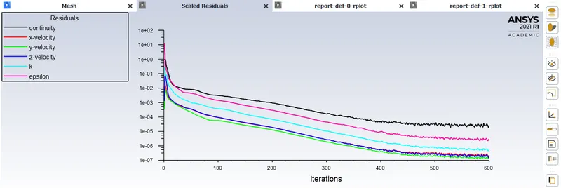
Residuals:
Console:

CFD Post:
Particle time:
Velocity:
Pressure:
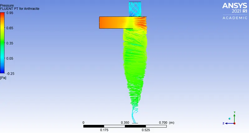
Swirling vortex:
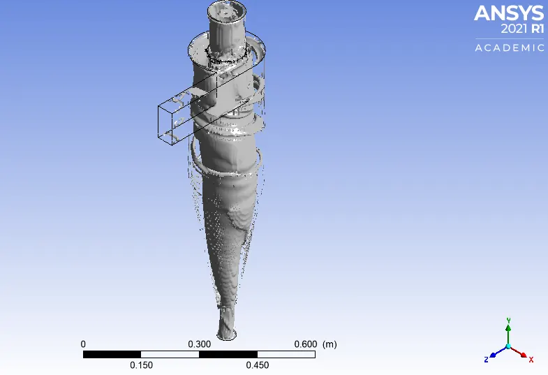
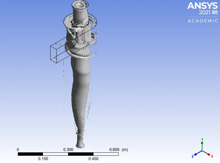
Animation: Video
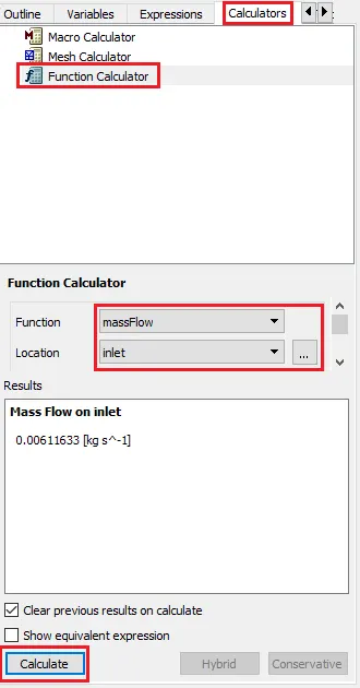
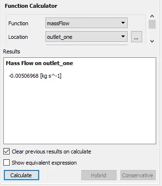
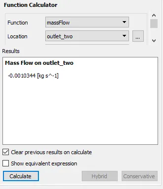
Other quantities:
3m/s, 5 micro meters:
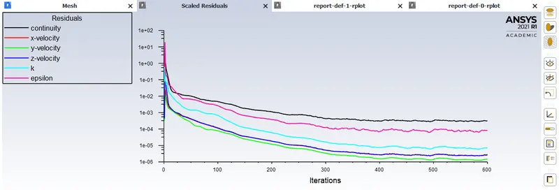
Residuals:
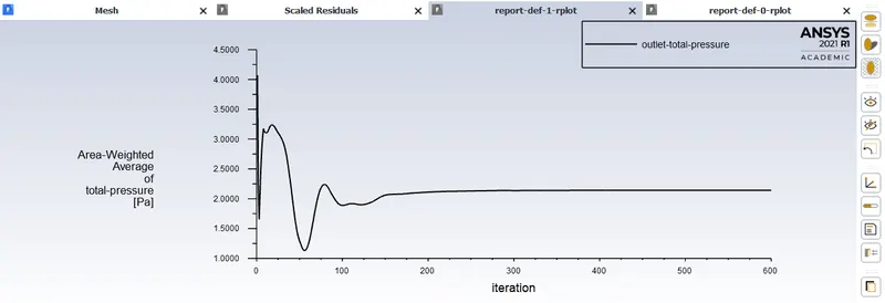
Plots:
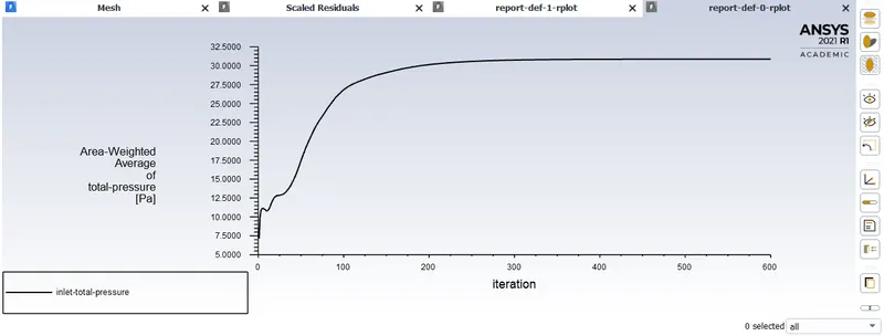
Console:
CFD Post:
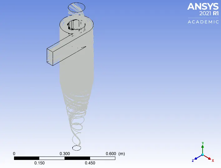
Particle time:
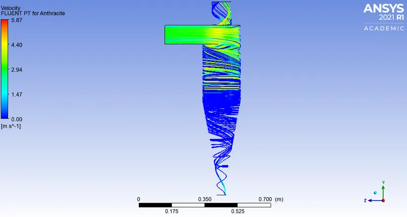
Velocity:
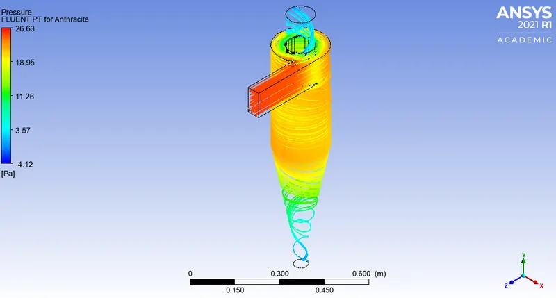
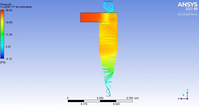
Pressure:
Swirling vortex:
Additional quantities:
5m/s, 5e-6:
Residuals:
Plots:
Console:

CFD Post:
Particle time:
Velocity:
Pressure:
Swirling Vortex:
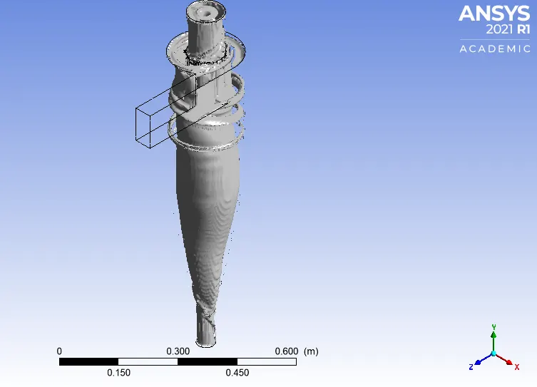
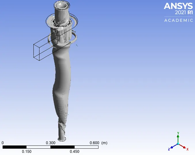
Animation:
Additional values:
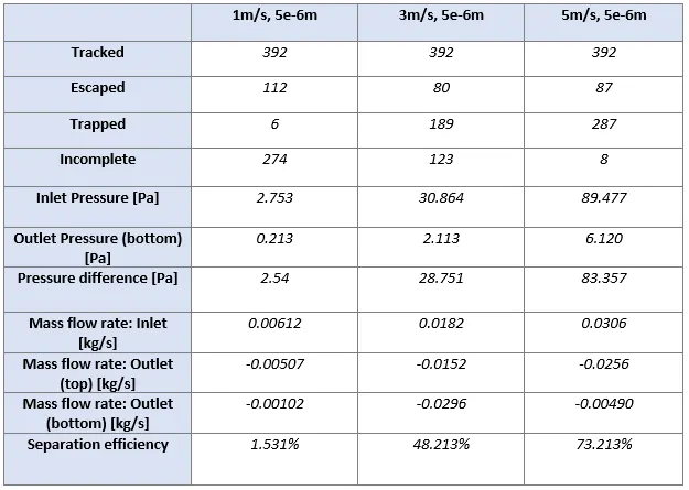
Tabulated results: Case 2
Conclusion:
Case 1:
CONCLUSION:
- Change in size of particle does'nt change the pressure at inlet and outlet.
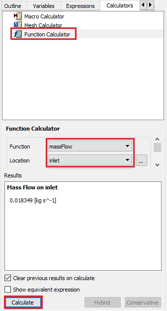
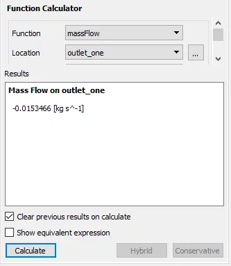
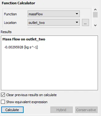
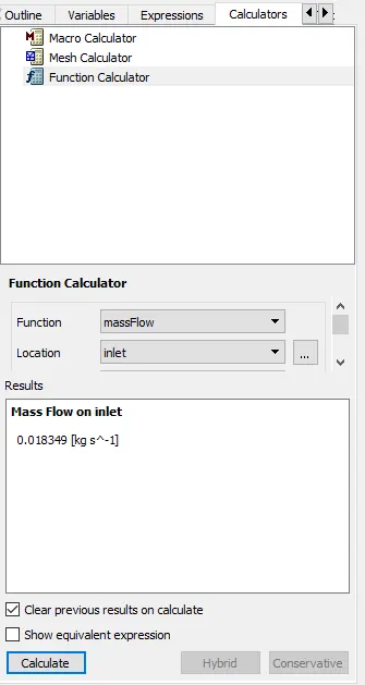
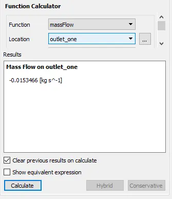
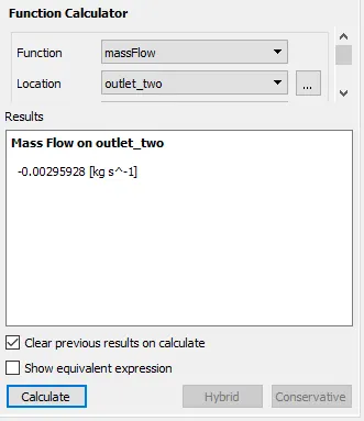
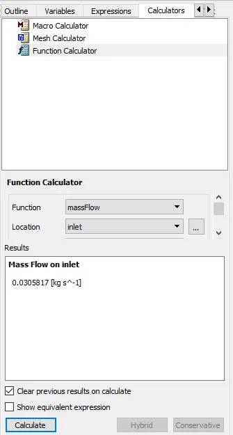
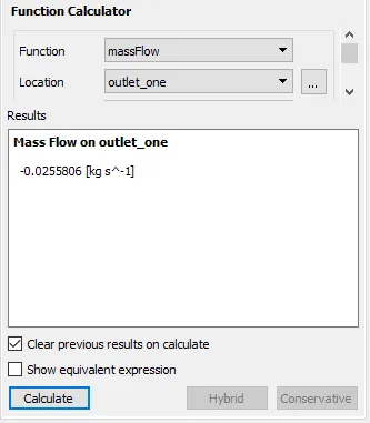
- The mass flow rate at inlet, outlet(top), outlet(bottom) remains same.
- As the size of the particle increases the number of trapped particles increase, this in turn increases the seperation effeciency.
- The number of escaped particles reduced as the size of the particulate increases.
Case 2:
CONCLUSION:
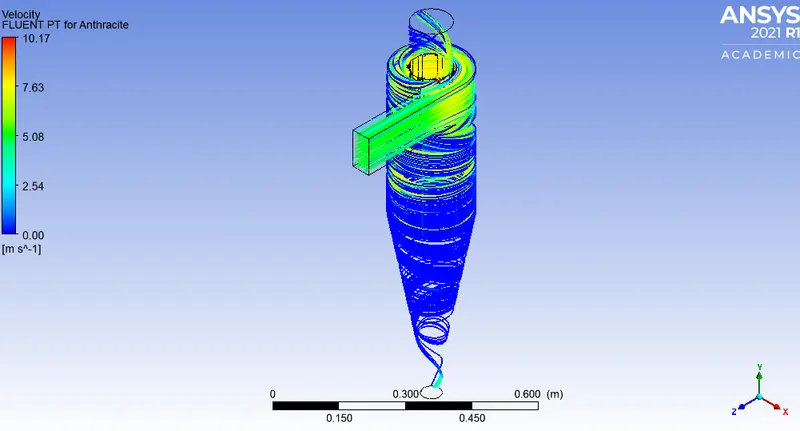
- With change in velocity at inlet and the size of the particles remaining same, the number of trapped particles also increases.
- The mass flow rate at inlet, outlet(top), outlet(bottom) changes dramatically.
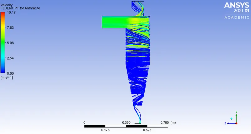
- As the size of the velocity increases the number of trapped particles increase, this in turn increases the seperation effeciency.
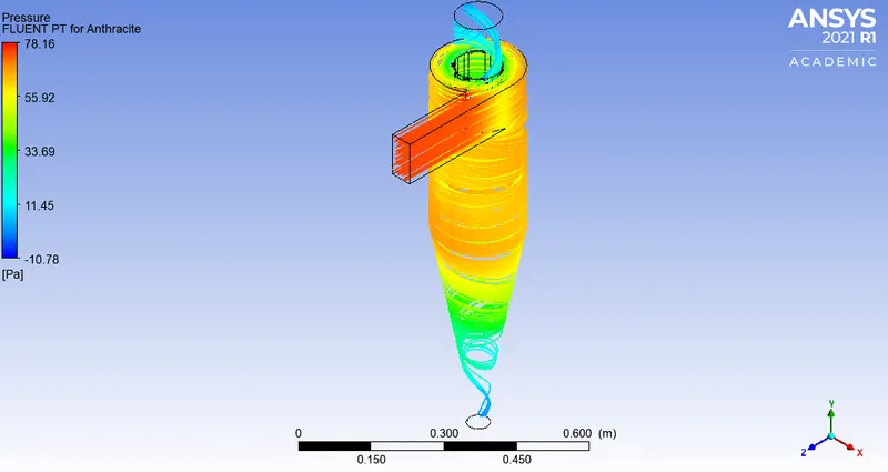
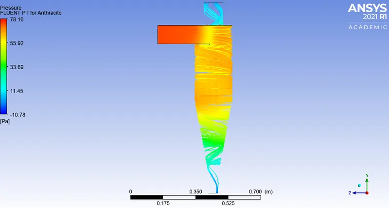
- The pressure at inlet and outlet increases with increase in temperature.
- With increase in velocity the number of incomplete particles decreases.
References:
Help for particle tracking data:
https://www.youtube.com/watch?v=9jIrgH2t8T4
DPM iteration interval:
Empirical models used to calculate the cyclone separator efficiency:
https://drive.google.com/file/d/1vJ0NxyMLNjbS3QAv4Tl_0Zoa9zjL_hdz/view?usp=sharing
https://nptel.ac.in/content/storage2/courses/103103027/pdf/mod5.pdf
Detailed theoretical study on cyclone seperator:
https://core.ac.uk/download/pdf/147123938.pdf
Other references:
https://drive.google.com/file/d/18tjkI67HDORCS_XYIjYB8dRhy14ix9lF/view?usp=sharing
https://drive.google.com/file/d/1GIjBrMIidaWfJYPzr8nYC67ain7WJKW3/view?usp=sharing
https://skill-lync.com/knowledgebase/theory-guide-for-discrete-phase-modelling