Basics of ML & AL Week 2 Challenge
1) Calculate all 4 business moments using pen and paper for the below data set.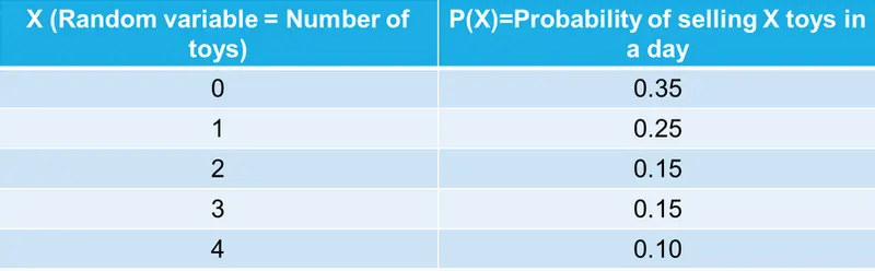
First business moment :
Measure of central tendency : Mean (`mu`) =`sum(x_i)*P(x)`
| x | P(x) | xi*P(x) | |
| 0 | 0.35 | 0 | |
| 1 | 0.25 | 0.25 | |
| 2 | 0.15 | 0.3 | |
| 3 | 0.15 | 0.45 | |
| 4 | 0.1 | 0.4 | |
| `sum` | 10 | 1 | 1.4 |
Mean (`mu`) =`sum(x_i)*P(x)`
= `0*0.35+1*0.25+2*0.15+3*0.15+4*0.1`
= 1.4
Second business moment :
Measure of variance`(sigma)^2` : `sum(x_i-mu)^2*P(x)`
| x | P(x) | xi*P(x) | `(x_i-mu)^2*P(x)` | |
| 0 | 0.35 | 0 | 0.686 | |
| 1 | 0.25 | 0.25 | 0.04 | |
| 2 | 0.15 | 0.3 | 0.054 | |
| 3 | 0.15 | 0.45 | 0.384 | |
| 4 | 0.1 | 0.4 | 0.676 | |
| `sum` | 10 | 1 | 1.4 | 1.84 |
Variance (`sigma^2`) = `sum(x_i-mu)^2*P(x)`
= `(0-1.4)^2*0.35+(1-1.4)^2*0.25+(2-1.4)^2*0.15+(3-1.4)^2*0.15+(4-1.4)^2*0.1`
= 1.84
Third business moment :
Skewness : sk =`sum((x_i-mu)/sigma)^3*P(x)`
| x | P(x) | xi*P(x) | (P(x)*(xi-mean)^2) | a=(xi-mean)/sqrt(sigma) | a^3*P(x) | |
| 0 | 0.35 | 0 | 0.686 | -1.032093693 | -0.384791453 | |
| 1 | 0.25 | 0.25 | 0.04 | -0.294883912 | -0.00641052 | |
| 2 | 0.15 | 0.3 | 0.054 | 0.442325868 | 0.012981303 | |
| 3 | 0.15 | 0.45 | 0.384 | 1.179535649 | 0.246163962 | |
| 4 | 0.1 | 0.4 | 0.676 | 1.91674543 | 0.704195604 | |
| Sum | 10 | 1 | 1.4 | 1.84 | 0.572138895 |
Variance (`sigma^2`)=1.84
`sigma = sqrt(1.84)`= 1.3565
sk = `sum((x_i-mu)/sigma)^3*P(x)`
= `((0-1.4)/1.3565)^3*0.35+((1-1.4)/1.3565)^3*0.25+((2-1.4)/1.3565)^3*0.15+((3-1.4)/1.3565)^3*0.15+((4-1.4)/1.3565)^3*0.10`
= 0.70413
Fourth business moment :
Kurtosis : kt =`sum((x_i-mu)/sigma)^4*P(x) - 3`
| x | P(x) | xi*P(x) | (P(x)*(xi-mean)^2) | a=(xi-mean)/sqrt(sigma) | a^3*P(x) | a^4*P(x) | |
| 0 | 0.35 | 0 | 0.686 | -1.032093693 | -0.384791453 | 0.39714083 | |
| 1 | 0.25 | 0.25 | 0.04 | -0.294883912 | -0.00641052 | 0.00189036 | |
| 2 | 0.15 | 0.3 | 0.054 | 0.442325868 | 0.012981303 | 0.00574197 | |
| 3 | 0.15 | 0.45 | 0.384 | 1.179535649 | 0.246163962 | 0.29035917 | |
| 4 | 0.1 | 0.4 | 0.676 | 1.91674543 | 0.704195604 | 1.34976371 | |
| Sum | 10 | 1 | 1.4 | 1.84 | 0.572138895 | 2.04489603 |
Variance (`sigma^2`)=1.84
`sigma = sqrt(1.84)`= 1.3565
kt =`sum((x_i-mu)/sigma)^4*P(x) - 3`
= `(((0-1.4)/1.3565)^4*0.35+((1-1.4)/1.3565)^4*0.25+((2-1.4)/1.3565)^4*0.15+((3-1.4)/1.3565)^4*0.15+((4-1.4)/1.3565)^4*0.10)-3`
= 2.04489603
| First business moment : Mean | 1.4 | |
| Second business moment : Variance | 1.84 | |
| Third business moment : sk | 0.572138895 | |
| Fourth business moment : kt |
(2.04489603024575)-3 |
-0.95510397 |
2)What is the significance of expected value when simple mean (Sum of all observations/number of observations) is already in place
Arithmetic mean is simple average of numbers not weighted by anything. However in Expected Value, the numbers are weighted by their probability.
When we consider the occourances of quantities to be same in experiment of calculating aritheatic mean and expected value then arithametic mean will give us same answer as the expected value .
Arithmetic mean : is the total of the sum of all values in a collection of numbers divided by the number of numbers in a collection. It is calculated in the following way:
`(x1+x2+x3+x4+......)/n`
x1,x2,x3.....=outcomes
n=number of outcomes
Example :
What is the Expected Value (EV)?
The expected value (EV) is an anticipated value for an investment at some point in the future. In statistics and probability analysis, the expected value is calculated by multiplying each of the possible outcomes by the likelihood each outcome will occur and then summing all of those values. By calculating expected values, investors can choose the scenario most likely to give the desired outcome.
`EV=sumx_i*P(x)`
Example :
In a development company. Your manager just asked you to assess the viability of future development projects and select the most promising one. According to estimates, Project A, upon completion, shows a probability of 0.4 to achieve a value of $2 million and a probability of 0.6 to achieve a value of $500,000. Project B shows a probability of 0.3 to be valued at $3 million and a probability of 0.7 to be valued at $200,000 upon completion.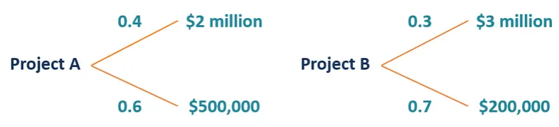
In order to select the right project, you need to calculate the expected value of each project and compare the values with each other. The EV can be calculated in the following way:
EV (Project A) = [0.4 × $2,000,000] + [0.6 × $500,000] = $1,100,000
EV (Project B) = [0.3 × $3,000,000] + [0.7 × $200,000] = $1,040,000
The EV of Project A is greater than the EV of Project B. Therefore, your company should select Project A.
The above examples tell us about all the difference between arithmetic mean and expected value .
3)Having skewness in the curve considered to be bad in the analysis?
Skewness :
Skewness refers to a distortion or asymmetry that deviates from the symmetrical bell curve, or normal distribution in a set of data. If the curve is shifted to the left or to the right, it is said to be skewed. Skewness can be quantified as a representation of the extent to which a given distribution varies from a normal distribution. A normal distribution has a skew of zero .
Why is skewness important ?
Linear models work on the assumption that the distribution of the independent variable and the target variable are similar. Therefore, knowing about the skewness of data helps us in creating better linear models.
Let’s take a look at the below distribution. It is the distribution of horsepower of cars: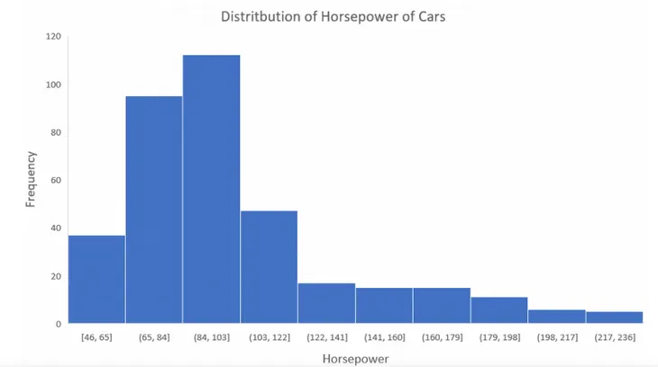
You can clearly see that the above distribution is positively skewed. Now, let’s say you want to use this as a feature for the model which will predict the mpg (miles per gallon) of a car.
Since our data is positively skewed here, it means that it has a higher number of data points having low values, i.e., cars with less horsepower. So when we train our model on this data, it will perform better at predicting the mpg of cars with lower horsepower as compared to those with higher horsepower.
You can see that our distribution is positively skewed and most of the outliers are present on the right side of the distribution.
Positively skewed :
A positively skewed distribution is the distribution with the tail on its right side. The value of skewness for a positively skewed distribution is greater than zero. As you might have already understood by looking at the figure, the value of mean is the greatest one followed by median and then by mode.
So why is this happening?
Well, the answer to that is that the skewness of the distribution is on the right; it causes the mean to be greater than the median and eventually move to the right.
Also, the mode occurs at the highest frequency of the distribution which is on the left side of the median. Therefore, mode < median < mean.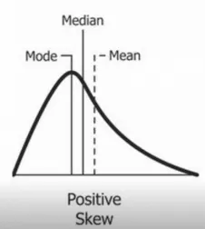
Negatively skewed :
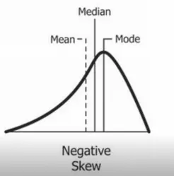
A negatively skewed distribution is the distribution with the tail on its left side. The value of skewness for a negatively skewed distribution is less than zero.
You can also see in the above figure that the mean < median < mode.
From the above we can understand that skewness doesn't have any bad effect on analysis rather it helps us identify certain characteristics of the data set just by looking at the graph .
This proves to be very effective in data analytics and has no bad effects associated with it .
4)Evaluate the probabilities for continuous normal distribution with given mean = 680 and standard deviation = 31
a)P(X<711)
b)P(X>740)
c)P(600<X<720)
d)P(X=720)
How to convert the X into a standard normal distribution in Z .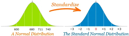
- The SND (i.e. z-distribution) is always the same shape as the raw score distribution. For example, if the distribution of raw scores if normally distributed, so is the distribution of z-scores.
- The mean of any SND always = 0.
- The standard deviation of any SND always = 1. Therefore, one standard deviation of the raw score (whatever raw value this is) converts into 1 z-score unit.
So , Z = `(X - mu)/ sigma`
where , `mu=mean`= 680
`sigma =`Standard deviation = 31
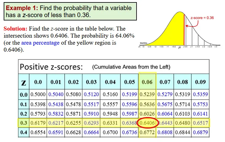
Z Table :
a)Converting P(X<711) into Z score ,
Z = `(X - mu)/ sigma`
= (711 - 680)/31
= 1
Since we converted X to Z and also 711 to 1 ,(X<711) converts to (Z<1)
From the Z table at Z=0
So , probablity is P(Z<1) = 0.8413
b)Converting P(X>740) into Z score ,
Z = `(X - mu)/ sigma`
= (740 - 680)/31
= 1.9355 ~ 1.94
Since we converted X to Z and also 711 to 1.94 ,(X>711) converts to (Z>1.94)
From the Z table at Z=0
So , probablity of Z<1.94 is P(Z<1.94) = 0.9738
But the probablity of Z>1.94 is P(Z>1.94) is (1-0.9738) = 0.0262
So ,P(Z>1.94) = 0.0262
c)Converting P(600<X<720) into Z score ,
Z = `(X - mu)/ sigma`
For X = 600 ,
Z = (600 - 680)/31
= -2.5805 ~ -2.57
Since we converted X to Z and also 600 to -2.57 ,(X>600) converts to (Z>-2.57)
From the Z table at Z=0
So , probability of Z>-2.57 is P(Z>-2.57) = 0.0051
Z = `(X - mu)/ sigma`
For X = 720 ,
Z = (720 - 680)/31
= 1.2903226 ~ 1.28
Since we converted X to Z and also 720 to 1.28 ,(X<720) converts to (Z<1.28)
From the Z table at Z=0
So , probability of Z<1.28 is P(Z<1.28) = 0.8997
The actual total probablity of P(600<X<720) is P(-2.57<Z<1.28)
which is 0.8997 - 0.0051 = 0.8946
d)P(X=720)
This is an interesting case of finding the probablity of an occourance within the range of 720 and 720 ,in other words would mean P(720<X<720) .
Z = `(X - mu)/ sigma`
For X = 720 ,
Z = (720 - 680)/31
= 1.2903226 ~ 1.29
So , probability of Z=1.29 is P(Z=1.29) = 0.8997
So,
P(1.3<Z<1.3)
= 0.8997-0.8997
=0
5)Explain the curve below .
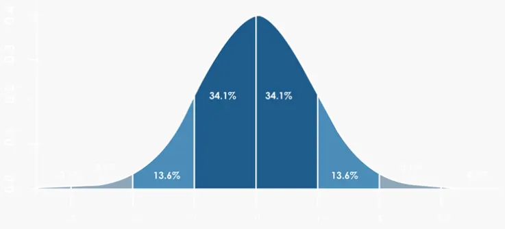
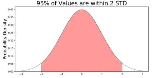
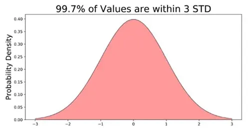
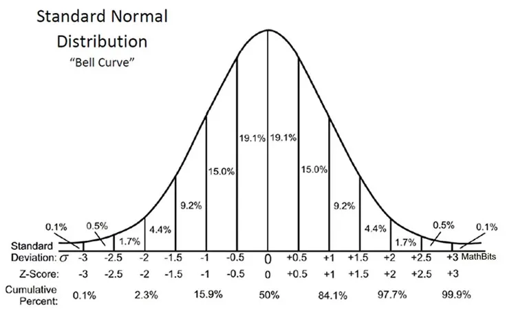
The above image show z scores on the horizontal axis and the probablity distribution on the vertical axis .
1.The value of the z-score tells you how many standard deviations you are away from the mean. If a z-score is equal to 0, it is on the mean.
2.A positive z-score indicates the raw score is higher than the mean average. For example, if a z-score is equal to +1, it is 1 standard deviation above the mean.
3.A negative z-score reveals the raw score is below the mean average. For example, if a z-score is equal to -2, it is 2 standard deviations below the mean.
4.Another way to interpret z-scores is by creating a standard normal distribution (also known as the z-score distribution or probability distribution).
Formula to find z scores :
`Z = (x-mu)/ sigma`
`sigma`= Standard deviation
`mu`= Mean
`x=`Value of x(value being examined)
a) The SND (i.e. z-distribution) is always the same shape as the raw score distribution. For example, if the distribution of raw scores if normally distributed, so is the distribution of z-scores.
b) The mean of any SND always = 0.
c) The standard deviation of any SND always = 1. Therefore, one standard deviation of the raw score (whatever raw value this is) converts into 1 z-score unit.
5. The SND allows researchers to calculate the probability of randomly obtaining a score from the distribution (i.e. sample).
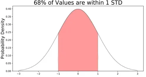
For example, there is a 68% probability of randomly selecting a score between -1 and +1 standard deviations from the mean .
The probability of randomly selecting a score between -1.96 and +1.96 standard deviations from the mean is 95%
6) What is kurtosis ?
Kurtosis is a statistical measure used to describe the degree to which scores cluster in the tails or the peak of a frequency distribution.
The peak is the tallest part of the distribution, and the tails are the ends of the distribution.
There are three types of kurtosis: mesokurtic, leptokurtic, and platykurtic.
- Mesokurtic: Distributions that are moderate in breadth and curves with a medium peaked height.
- Leptokurtic: More values in the distribution tails and more values close to the mean (i.e. sharply peaked with heavy tails)
- Platykurtic: Fewer values in the tails and fewer values close to the mean (i.e. the curve has a flat peak and has more dispersed scores with lighter tails).
When kurtosis is equal to 0, the distribution is mesokurtic. This means the kurtosis is the same as the normal distribution, it is mesokurtic (medium peak).
The kurtosis of a mesokurtic distribution is neither high nor low, rather it is considered to be a baseline for the two other classifications.
Negative values of kurtosis indicate that a distribution is flat and has thin tails. Platykurtic distributions have negative kurtosis values.
A platykurtic distribution is flatter (less peaked) when compared with the normal distribution, with fewer values in its shorter (i.e. lighter and thinner) tails.
Positive values of kurtosis indicate that a distribution is peaked and possess thick tails. Leptokurtic distributions have positive kurtosis values.
A leptokurtic distribution has a higher peak and taller (i.e. fatter and heavy) tails than a normal distribution.
An extreme positive kurtosis indicates a distribution where more of the values are located in the tails of the distribution rather than around the mean.