Week 7 - Simulation of a 1D Super-sonic nozzle flow simulation using Macormack Method
Subsonic and supersonic isentropic flow :
We consider the steady state ,isemtropic flow through a convergent-divergent nozzle as shown in the figure below.The flow of the inlet comes from a reservoir where the pressure and temprature are denoted by `p_0` & `T_0` respectively .The crossectional area of the reservir is large (`A-> oo`) and hence velocity is very small (`V->0`) .`p_0`& `T_0` are thus known as stagnation values or total pressure or total temprature .
The flow expands isentropically at the end of the nozzle at supersonic speeds where exit temprature ,pressure ,velocity & mach number are denoted by `T_e`,`p_e`,`V_e`& `M_e`respectively.The flow is locally subsonic in the convergent section of the nozzle,sonic (M=1) at the throat & supersonic at the divergent section of the nozzle .
This is a 2d flow in reality but we assume that the flow varies only in the x direction so hence the name quasi 1d flow.
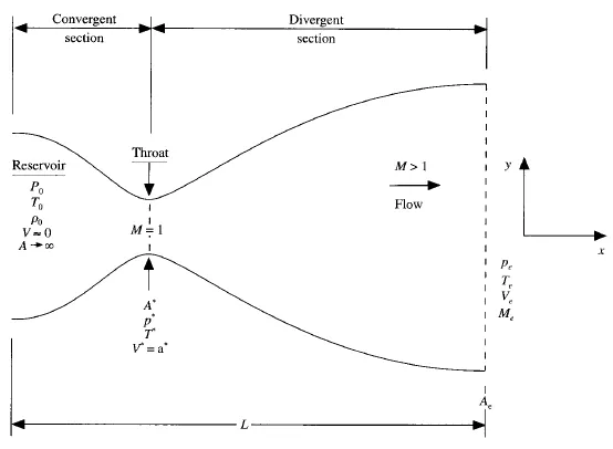
fig(1) schematic for subsonic and suoersonic isentropic nozzle flow.
MACCORMACK'S TECHNIQUE
- Variant of Lax-Wendroff approach but is simpler in it's application.
- It is an explicit finite difference technique which is second order accurate .
- We assume that we know all the flow field in each grid point shown in fig(4) at time step t and we proceed to calculate the flow field variables at time t+dt.
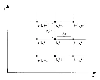
Fig(4) : Rectangular grid segment 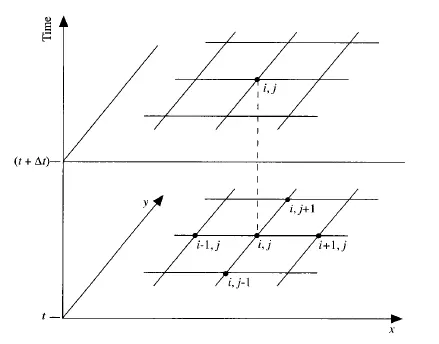
Fig(5) : A schematic for time marching
First consider the density at grid point (i,j) at time t+dt. In Maccormack method this can be obtained from the below equations .
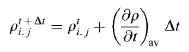
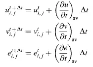
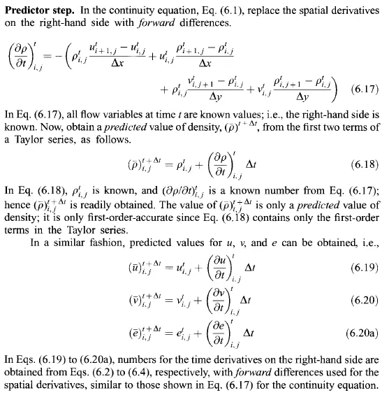
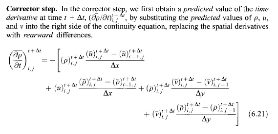
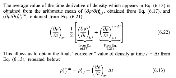
In Maccormack technique , the use of forward differences on the predictor & backward differences on the corrector is not sacrosanct .The same order of accuracy is obtained by using backward differences on the predictor and forward differences on the corrector .
Non conservation form
1. Continuity equation :
Let us consider the continuity equation in control volume fixed in space to the shaded region in fig(2).
The shaded region is the control volume which is a slice of the nozzle flow of thickness 'dx'.
Fig(2) clearly denotes the inlet and outlet variables ,on the left of the shaded region is the inlet flow variables & on the right hand side of the shaded region is the flow variables at outlet of nozzle.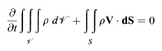
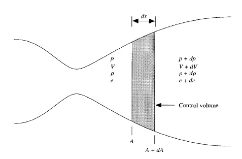
fig(2):control volume derived from partial differential equations for unsteady ,quasi 1d flow.
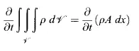
The volume integral in the above equation can be written in terms of A(area) & dx is given below.
The surface integral can be written as 
The negative sign in the first term of RHS is because the inlet vector is opposite to the area vector of the control volume.
The above equation can be further simplified as,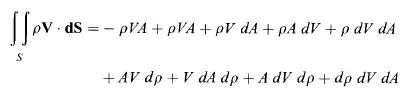
Now in the above equation we ignore all the product of differentials as their values are almost insignificant .
Substitute the surface integral and volume integral into the original continuity equation and results to this equation.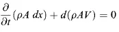
Now further dividing the above equation by 'dx'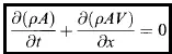
The above equation is the non conservative form of the continuity equation .
2. Momentum equation :
The integral form of x component of the moemntum equation for invicid flow with no body forces is given below .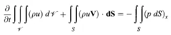
The time derivatie of the volume integral can be written in the below given form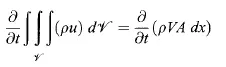
The surface integral can also be written as,
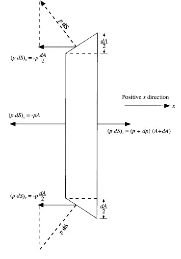
fig(3):sign convection for forces acting in the x direction on the control volume.
The RHS of the first equation from this section can also be written as the following,
The term dA/2 is because of top and bottom inclined faces of the control volume.
Combining the time derivatie of the volume integral,surface integral & RHS term must be substituted in the momentum equation
Ignoring the products of integrals 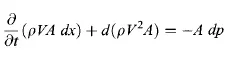
divide the above equation by dx on both sides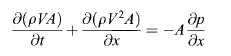
The above equation is the conservative form of the momentum equation .
Now consider the continuity equation for non conservative form from above section and multiply it by V on both sides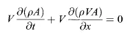
Subtract the above equation with the conservative form of continuity equation to obtain the below equation.
further simplify the above equation and divide by A on both sides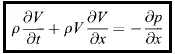
The above equation is the non conservative form of the momentum equation .
3. Energy equation :
Let's consider the integral form of energu=y equation ,for adiabatic flow with no body forces and no viscous effects.
Considering the sign convention to the control volume from fig(3) 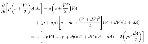
Ignoring the product of differentials and then further simplifying the above equation we get,
Further ,
As dx approaches zero the above equation becomes 
The above equation is the conservative form of the energy equation for unsteady, quasi 1d flow expressed in terms of e .
The non conservative form of the energy equation is derived from the conservative form of momentum equation .
Now multiply this equation by V on both sides .
Subtracting the above equation with the conservative form of the energy equation .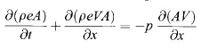
The above equation is the conservative form of the energy equation for quasi 1d flow.
Consider the continuity equation of the nonconservative form we derived in section 1 and multiply it by e on both sides .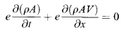
Subtract the above equation with the conservative form of the energy equation for quasi 1d flow.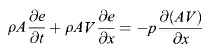
Expanding the RHS & divide by A on both sides 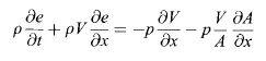
Further simplified into 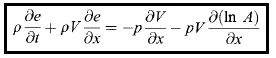
This is the nonconservative form of energy equation expressed in terms of internal energy ,appropriate to unsteady ,quasi 1d flow.
Non dimentional nonconservative equations are given below after mathetical manipulation.
Coninuity Equation :
Momentum Equation :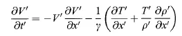
Energy Equation :
The finite difference equations for the same is given below


CALCULATION OF TIME STEP :
The present application to subsonic-supersonic isentropic nozzle flow is governed by non linear partial differential equations
here ,V=local flow velocityat a point in the flow
a=local speed of sound 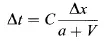
at a given gridpoint i
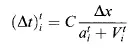
at the adjacent grid point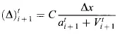
we have to choose the minimum value of dt and then use it in out code to get a time accurate solution.
We have found from the textbook that dt=0.0267 is the least value of dt so we are proceeding with it .
Here we consider a(speed of sound in the medium)=`sqrt(Temprature)`
This we obtained from a=`sqrt(gamma*R*Temprature)`
where,`gamma=1`& `R=1`.
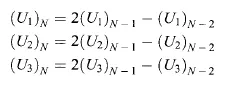
BOUNDARY CONDITIONS
The theory of characteristics says that only one variable must be specified and the other must be allowed to float at the inlet so based on the slope of the line we declare the boundary condition for inlet by method of interpolation.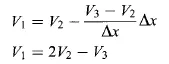

The outlet boundary condition needs 2 values to be floating by the theory of characteristics .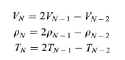
Nozzle shape and initial conditions

Mach number.
M=flow velocity of a fluid past a boundary/speed of sound in that medium
M=V/a
a=`sqrt(gamma*R*Temprature)`
where ,`gamma=1`& `R=1`.
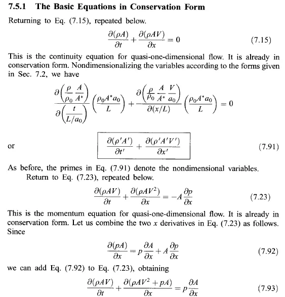
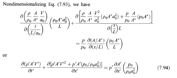
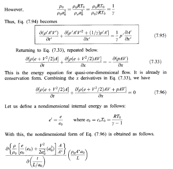
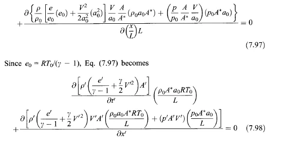
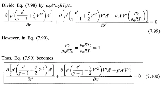
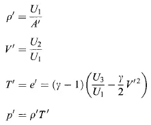
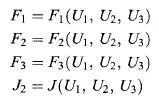
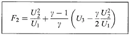
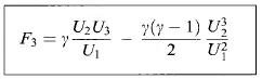
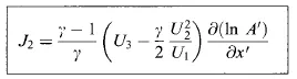
Equation (7.91),(7.95) & (7.100) are the non dimensional conservative form of continuity ,momentum & energy equations for quasi 1d flow respectively .
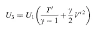
Additional formulas used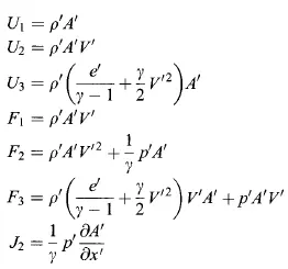
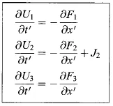

Boundary conditions :

Initial conditions :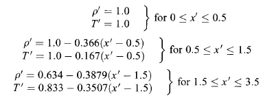
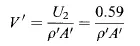
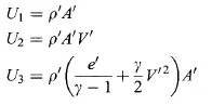
Time step dt=0.0267
Main code :
clear all
close all
clc

% inputs
n=31;
x=linspace(0,3,n);
dx=x(2)-x(1);
gamma=1.4;
% area
a=1+(2.2)*(x-1.5).^2;    % refer jd anderson table 7.1 for a'(a transpose) values & compare them

th = find(a==1);
%Non conservative function
[rho_nc,t_nc,v_nc,m_nc,p_nc,M_nc] = main_nonconservative(n,x,dx,gamma,a,th);
%conservative function
[rho_c,v_c,t_c,p_c,m_c,M_c,U1,U2,U3] = main_conservative(n,x,dx,gamma,a,th);

figure(7)
plot(x,m_nc,'r')
hold on
plot(x,m_c)
legend('massflow rate non conservative','massflow rate conservative')
xlabel('x')
ylabel('mass flow rate')
title('mass flow rate plot')
Function code : Nonconservation form
function [rho,t,v,m,p,M] = main_nonconservative(n,x,dx,gamma,a,th)

% calculate initial profiles
rho=1-0.3146*x;
t=1-0.2314*x;
% remember Temprature T & x are arrays so we must use dot(.) and star(*) to
% do the elementwise operator
v=(0.1+1.09*x).*t.^0.5;

nt=1400;
% arbitrary time step ,use courant number criteria in challenge
dt=0.0201;

% outer time loop
for k=1:nt
    rho_old=rho;
    v_old=v;
    T_old=t;
%     predictor method

% forward differencing the space terms on rhs and then compute time step
% continuity equation : to be solved on the inner nodes only
% loop for inner nodes
for j=2:n-1
%     drho_dt_p=-rho(j)*(v(j+1)-v(j))/dx-rho(j)*v(j)*(log(a(j+1)-log(a(j))))/dx-v(j)*(rho(j+1)-rho(j))/dx;
% frequently repeated difference values form the continuity equation
dvdx=(v(j+1)-v(j))/dx;
drhodx=(rho(j+1)-rho(j))/dx;
dTdx=(t(j+1)-t(j))/dx;
dlogadx=(log(a(j+1))-log(a(j)))/dx;

% combined continuity equation
drhodt_p(j)=-rho(j)*dvdx-rho(j)*v(j)*dlogadx-v(j)*drhodx;
% combined momentum equation
dvdt_p(j)=-v(j)*dvdx-(1/gamma)*(dTdx+t(j)/rho(j))*drhodx;
% combined energy equation
dTdt_p(j)=-v(j)*dTdx-(gamma-1)*t(j)*(dvdx+v(j)*dlogadx);

   % solution update
rho(j)=rho(j)+drhodt_p(j)*dt;
v(j)=v(j)+dvdt_p(j)*dt;
t(j)=t(j)+dTdt_p(j)*dt;

end

% v=v+dvdt_p*dt; caused error because the matrix dimensions do not match.

for j=2:n-1
%     corrector method

%     drho_dt_p=-rho(j)*(v(j+1)-v(j))/dx-rho(j)*v(j)*(log(a(j+1)-log(a(j))))/dx-v(j)*(rho(j+1)-rho(j))/dx;
% frequently repeated difference values form the continuity equation
dvdx=(v(j)-v(j-1))/dx;
drhodx=(rho(j)-rho(j-1))/dx;
dTdx=(t(j)-t(j-1))/dx;
dlogadx=(log(a(j))-log(a(j-1)))/dx;

% combined continuity equation
drhodt_c(j)=-rho(j)*dvdx-rho(j)*v(j)*dlogadx-v(j)*drhodx;
% combined momentum equation
dvdt_c(j)=-v(j)*dvdx-(1/gamma)*(dTdx+t(j)/rho(j))*drhodx;
% combined energy equation
dTdt_c(j)=-v(j)*dTdx-(gamma-1)*t(j)*(dvdx+v(j)*dlogadx);

end
% calculating average time derivative
drhodt=0.5*(drhodt_p+drhodt_c);
dvdt=0.5*(dvdt_p+dvdt_c);
dTdt=0.5*(dTdt_p+dTdt_c);

% final update of the solution
for i=2:n-1
% final solution update : error because of not updating old values on rhs
% rho(i)=rho(i)+drhodt(i)*dt;
% v(i)=v(i)+dvdt(i)*dt;
% T(i)=T(i)+dTdt(i)*dt;
rho(i)=rho_old(i)+drhodt(i)*dt;
v(i)=v_old(i)+dvdt(i)*dt;
t(i)=T_old(i)+dTdt(i)*dt;
end

% boundary conditions
% inlet
v(1)=2*v(2)-v(3);
% outlet
v(n)=2*v(n-1)-v(n-2);
rho(n)=2*rho(n-1)-rho(n-2);
t(n)=2*t(n-1)-t(n-2);

m = rho.*a.*v;
p = rho.*t;
M = v./sqrt(t);


 figure(1)
  if k==1
     plot(x,m)
     hold on
  end
  if k==10
     plot(x,m)
     hold on
  end
  if k==50
     plot(x,m)
     hold on
  end
  if k==100
     plot(x,m)
     hold on
  end
  if k==400
     plot(x,m)
     hold on
  end
  if k==600
     plot(x,m)
     hold on
  end
  if k==800
     plot(x,m)
     hold on
  end
  if k==1000
     plot(x,m)
     hold on
  end
  if k==1400
     plot(x,m)
     hold on
  end
  hold on
  xlabel('x')
  ylabel('m')

  rho_th(k) = rho(th);
  v_th(k) = v(th);
  t_th(k) = t(th);
  p_th(k) = p(th);
  M_th(k) = M(th);


end
legend('1dt','10dt','50dt','100dt','400dt','600dt','800dt','1000dt','1400dt')
title('Variation of flow rate at different timesteps')

figure(2)
%steady state plot
subplot(5,1,1)
plot(x,rho)
xlabel('x')
ylabel('rho-density')
subplot(5,1,2)
plot(x,v)
xlabel('x')
ylabel('v-velocity')
subplot(5,1,3)
plot(x,t)
xlabel('x')
ylabel('t-temprature')
subplot(5,1,4)
plot(x,M)
xlabel('x')
ylabel('M-Mach number')
subplot(5,1,5)
plot(x,p)
xlabel('x')
ylabel('p-pressure')
suptitle('steady state plot - Non conservative')
%
figure(3)
%Transient state plot at throat
subplot(5,1,1)
plot(rho_th)
xlabel('number of iterations')
ylabel('rho-density')
subplot(5,1,2)
plot(v_th)
xlabel('number of iterations')
ylabel('v-velocity')
subplot(5,1,3)
plot(t_th)
xlabel('number of iterations')
ylabel('t-temprature')
subplot(5,1,4)
plot(M_th)
xlabel('number of iterations')
ylabel('M-mach number')
subplot(5,1,5)
plot(p_th)
xlabel('number of iterations')
ylabel('p-pressure')
suptitle('Transient state plot(throat) - Non conservative')

end
Function code : Conservation form
function [rho,v,t,p,m,M,U1,U2,U3] = main_conservative(n,x,dx,gamma,a,th)

nt=1400;
% from text
dt=0.0267;

for i=1:n
    if x(i)>=0 && x(i)<=0.5
        rho(i)=1;
        t(i)=1;
    elseif x(i)>= 0.5 && x(i)<= 1.5
        rho(i)=1-0.366*(x(i)-0.5);
        t(i)=1-0.167*(x(i)-0.5);
    elseif x(i)>1.5 && x(i)<=3.5
        rho(i)=0.634-0.3879*(x(i)-1.5);
        t(i)=0.833-0.3507*(x(i)-1.5);
    end
end

v=0.59./(rho.*a);
m=rho.*v.*a;


U1=rho.*a;
U2=rho.*a.*v;
U3=U1.*((t/(gamma-1))+(gamma/2)*v.^2);

for k=1:nt

    U1_old=U1;
    U2_old=U2;
    U3_old=U3;

    F1=U2;
    F2=(U2.^2./U1)+((gamma-1)/(gamma))*(U3-0.5*gamma*(U2.^2./U1));
    F3=((gamma*U2.*U3)./U1)-(((gamma)*(gamma-1))*0.5)*(U2.^3./U1.^2);


%   predictor step
    for j=2:n-1
dadx = (a(j+1)-a(j))/dx;
J2(j)=(1/gamma)*(rho(j)*t(j))*dadx;

% continuity equation : conservative
dU1dt_p(j)=-(F1(j+1)-F1(j))/dx;
% momentum equation : conservative
dU2dt_p(j)=-((F2(j+1)-F2(j))/dx)+J2(j);
% energy equation : conservative
dU3dt_p(j)=-(F3(j+1)-F3(j))/dx;

% solution update
U1(j)=U1(j)+dU1dt_p(j)*dt;
U2(j)=U2(j)+dU2dt_p(j)*dt;
U3(j)=U3(j)+dU3dt_p(j)*dt;
end

F1=U2;
F2=(U2.^2./U1)+((gamma-1)/(gamma))*(U3-0.5*gamma*(U2.^2./U1));
F3=((gamma*U2.*U3)./U1)-(((gamma)*(gamma-1))*0.5)*(U2.^3./U1.^2);

rho=U1./a;
v=U2./U1;
t=(gamma-1).*((U3./U1)-0.5*(gamma)*v.^2);
p=rho./t;

%     corrector step
    for j=2:n-1
    dadx = (a(j)-a(j-1))/dx;
    J2(j)=(1/gamma)*(rho(j)*t(j))*dadx;


% continuity equation : conservative
dU1dt_c(j)=-(F1(j)-F1(j-1))/dx;
% momentum equation : conservative
dU2dt_c(j)=-((F2(j)-F2(j-1))/dx)+J2(j);
% energy equation : conservative
dU3dt_c(j)=-(F3(j)-F3(j-1))/dx;

end
%     average time values = 0.5*(predictor + corrector)
    dU1dt=0.5*(dU1dt_p+dU1dt_c);
    dU2dt=0.5*(dU2dt_p+dU2dt_c);
    dU3dt=0.5*(dU3dt_p+dU3dt_c);

%     final values
    for i=2:n-1

        U1(i)=U1_old(i)+dU1dt(i)*dt;
        U2(i)=U2_old(i)+dU2dt(i)*dt;
        U3(i)=U3_old(i)+dU3dt(i)*dt;

    end

% boundary conditions

% inlet
% fixed values for T & rho
U1(1)=a(1)*rho(1);
% calculation by exrtapolation
U2(1)=2*U2(2)-U2(3);
% floating value for velocity(v)
v(1)=U2(1)/U1(1);
U3(1)=U1(1)*((t(1)/(gamma-1))+(gamma/2)*(v(1)^2));

% outlet
% by interpolating we get
U1(n)=2*U1(n-1)-U1(n-2);
U2(n)=2*U2(n-1)-U2(n-2);
U3(n)=2*U3(n-1)-U3(n-2);


rho=U1./a;
v=U2./U1;
t=(gamma-1).*((U3./U1)-0.5*(gamma)*v.^2);
p=rho./t;
m= rho.*a.*v;
% mach number
M=v./sqrt(t);

  rho_th(k) = rho(th);
  v_th(k) = v(th);
  t_th(k) = t(th);
  p_th(k) = p(th);
  M_th(k) = M(th);

  figure(4)
  if k==1
     plot(x,m)
     hold on
  end
  if k==10
     plot(x,m)
     hold on
  end
  if k==50
     plot(x,m)
     hold on
  end
  if k==100
     plot(x,m)
     hold on
  end
  if k==400
     plot(x,m)
     hold on
  end
  if k==600
     plot(x,m)
     hold on
  end
  if k==800
     plot(x,m)
     hold on
  end
  if k==1000
     plot(x,m)
     hold on
  end
  if k==1400
     plot(x,m)
     hold on
  end
  hold on
  xlabel('x')
  ylabel('m')


end
legend('1dt','10dt','50dt','100dt','400dt','600dt','800dt','1000dt','1400dt')
title('Variation of flow rate at different timesteps')

figure(5)
%steady state plot
subplot(5,1,1)
plot(x,rho)
xlabel('x')
ylabel('rho-density')
subplot(5,1,2)
plot(x,v)
xlabel('x')
ylabel('v-velocity')
subplot(5,1,3)
plot(x,t)
xlabel('x')
ylabel('t-temprature')
subplot(5,1,4)
plot(x,M)
xlabel('x')
ylabel('M-mach number')
subplot(5,1,5)
plot(x,p)
xlabel('x')
ylabel('p-pressure')
suptitle('Transient state plot - Conservative')

figure(6)
%Transient state plot at throat
subplot(5,1,1)
plot(rho_th)
xlabel('number of iterations')
ylabel('rho-density')
subplot(5,1,2)
plot(v_th)
xlabel('number of iterations')
ylabel('v-velocity')
subplot(5,1,3)
plot(t_th)
xlabel('number of iterations')
ylabel('t-temprature')
subplot(5,1,4)
plot(M_th)
xlabel('number of iterations')
ylabel('M-mach number')
subplot(5,1,5)
plot(p_th)
xlabel('number of iterations')
ylabel('p-pressure')
suptitle('Transient state plot(throat) - Conservative')

end
Outputs :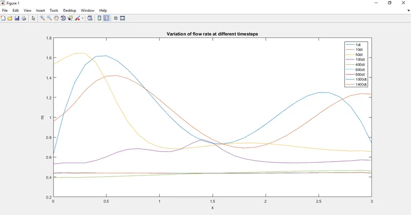
The above plot compares the values of mass for each different time step along the length of the nozzle .
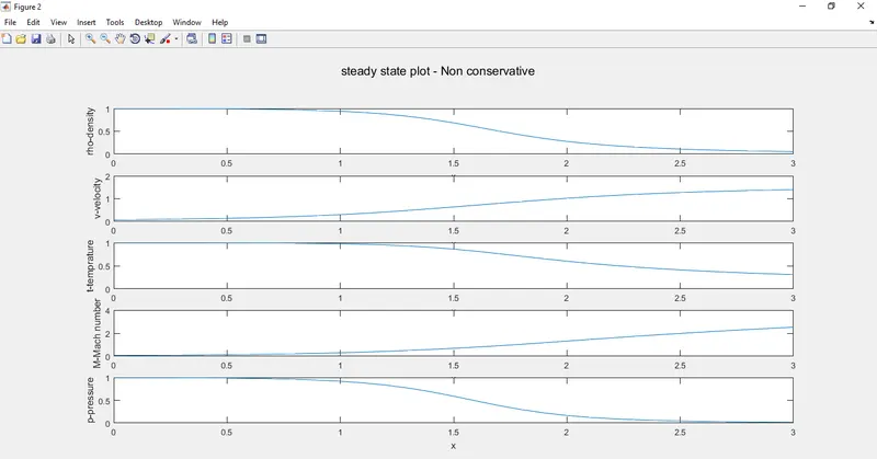
The above plot compares the variation of primitive variables over the entire length of the nozzle .
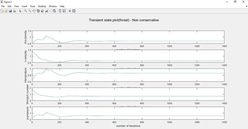
The above plot compares the variation in the values of primitive variables at the throat of the nozzle as the iterations progresses .
Note that the plots of all the primitive variables are unsteady at lower time steps and as the time steps increase the primitive values attain steady state.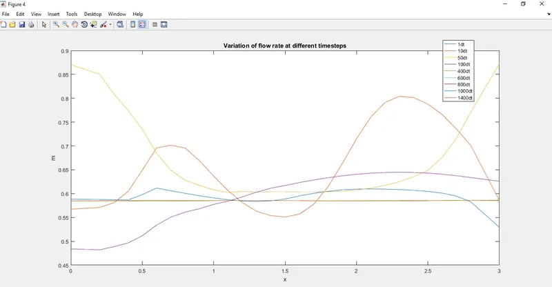
The above plot compares the values of mass for each different time step along the length of the nozzle .
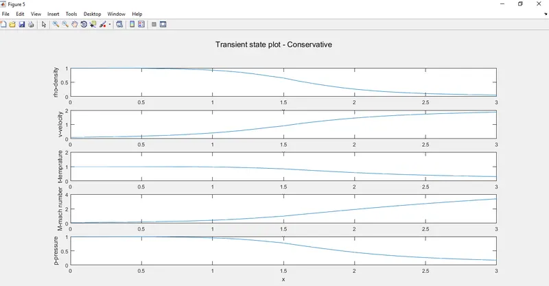
The above plot compares the variation of primitive variables over the entire length of the nozzle .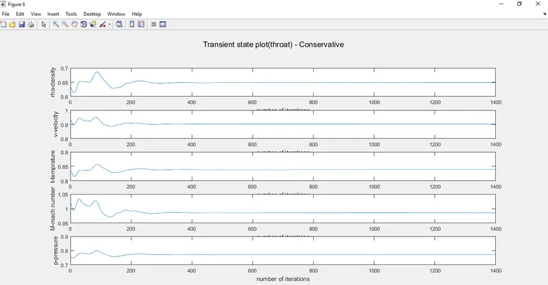
The above plot compares the variation in the values of primitive variables at the throat of the nozzle as the iterations progresses .
Note that the plots of all the primitive variables are unsteady at lower time steps and as the time steps increase the primitive values attain steady state.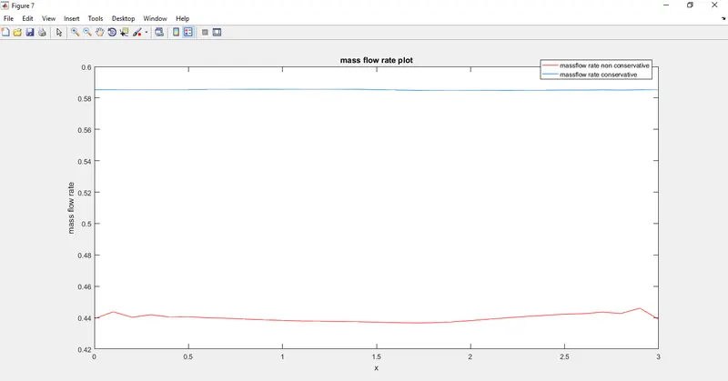
Comparison of Normalized mass flow rate distributions of both forms at different time steps.
Tabulated values for primitive variables from the program in comparison with values of the primitive variables from textbook (John D Anderson)
1 . Nonconservation form from matlab program after 1400 time steps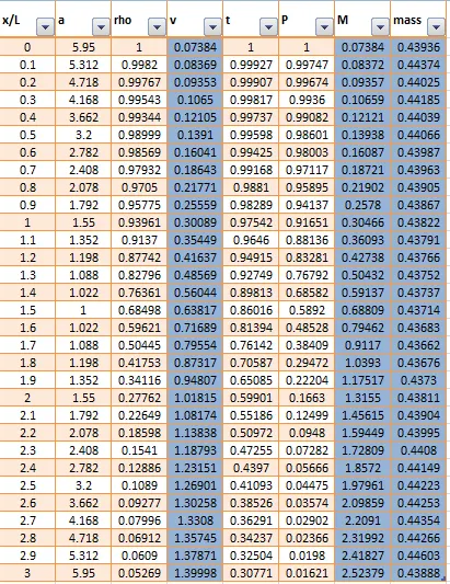
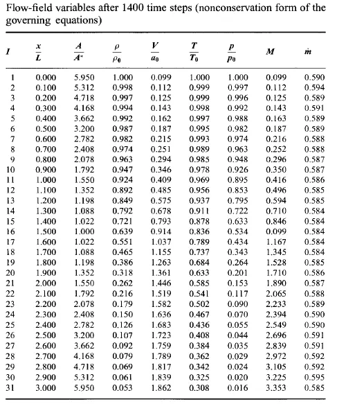
Note that the columns in blue is hughlightened because the values of the primitive variables do not match with the values nfrom the textbook .
2 . Conservation form from matlab program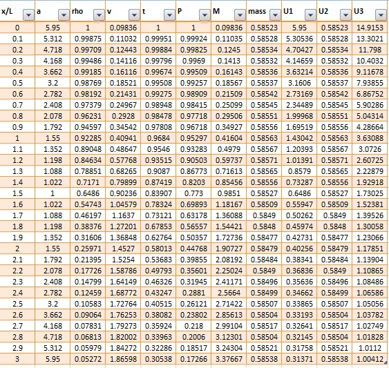
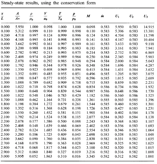
Note that all the values of the primitive variables match the values given from the textbook .
CONCLUSION :
Most of the results obtained from the matlab code for 1D Super-sonic nozzle flow using Maccormack method matches with the results given in J D Anderson - Computational fluid dynamics : the basics with application .