Supervised Learning - Classification Week 8 Challenge

Knn algorithm:

KNN is a simple algorithm, based on the local minimum of the target function which is used to learn an unknown function of desired precision and accuracy. The algorithm also finds the neighborhood of an unknown input, its range or distance from it, and other parameters. It’s based on the principle of “information gain”—the algorithm finds out which is most suitable to predict an unknown value.

KNN is widely known as an ML algorithm that doesn’t need any training on data. This is much different from eager learning approaches that rely on a training dataset to perform predictions on unseen data. With KNN, you don’t need a training phase at all.

KNN relies on observable data similarities and sophisticated distance metrics to generate accurate predictions. This technique may seem a bit counterintuitive and not trustworthy at first, but it’s actually very reliable. It’s popular in many fields, including:

1. Apply knn to the “Surface defects in stainless steel plates” and identify the differences

Code:

Dataset: https://docs.google.com/spreadsheets/d/1NyfH85JXo1L1qiryKB5qr3yTXIMTxHkFo1w3OLB942k/edit?usp=sharing

1. All the necessary libraries are imported and the dataset is imported.
2. To view the distribution of data of factors influencing a certain type of defect a histogram plot has been used to visualise the data.
3. The data is split into factors and defets.
4. The data has been manipulated to form a label encoded dataframe from the perviously existant one hot encoded data for the type of defects.
5. knn library along with the data splitter from sklearn has been called.
6. A for loop plots the accuracy plot of test and train data for knn
7. Confusion matrix is created along with a heat map to visualise the data classification accuracy.
8. Other classifiers like SVM, Decision tree and random forest have been used to show the level of accuracy each algorithm can produce.

import numpy as np
import pandas as pd
import matplotlib.pyplot as plt
import seaborn as sn
import scipy.stats as stats

data = pd.read_csv(r'E:ai mlaiml challengechallengesweek7faults.csv')
data.hist()
plt.show()
factors=data.iloc[:, 0:27]
df=data.iloc[:, 27:34]

corrmat = data.corr()
f, ax = plt.subplots(figsize=(10,10))
sn.heatmap(corrmat, ax=ax, cmap="YlGnBu", linewidths = 0.1)
plt.show()

pd.set_option('display.max_columns', None)
#pd.set_option('display.max_rows', None)
factors_zscore = stats.zscore(factors)

df['Class']=0
df['DefType']=''
#data Consolidation - Consolidating the target dummy variables into single variable
df.loc[df.Pastry==1,'Class'] = 1
df.loc[df.Z_Scratch==1,'Class'] = 2
df.loc[df.K_Scatch==1,'Class'] = 3
df.loc[df.Stains==1,'Class'] = 4
df.loc[df.Dirtiness==1,'Class'] = 5
df.loc[df.Bumps==1,'Class'] = 6
df.loc[df.Other_Faults==1,'Class'] = 7

#data Consolidation - Consolidating the target dummy variables into single variable
df.loc[df.Pastry==1,'DefType'] = 'Pastry'
df.loc[df.Z_Scratch==1,'DefType'] = 'Z_Scratch'
df.loc[df.K_Scatch==1,'DefType'] = 'K_Scatch'
df.loc[df.Stains==1,'DefType'] = 'Stains'
df.loc[df.Dirtiness==1,'DefType'] = 'Dirtiness'
df.loc[df.Bumps==1,'DefType'] = 'Bumps'
df.loc[df.Other_Faults==1,'DefType'] = 'Other_Faults'

df.drop(['Pastry','Z_Scratch','K_Scatch','Stains','Dirtiness','Bumps','Other_Faults','DefType'], axis=1, inplace=True)
print(df.describe())
print(df.head())

print(df)
print(factors)
print(factors.describe())
print(factors.head())

from sklearn.neighbors import KNeighborsClassifier
from sklearn.model_selection import train_test_split
X_train, X_test, y_train, y_test = train_test_split(factors_zscore, df, test_size = 0.2, random_state=0)
knn = KNeighborsClassifier(n_neighbors=7)
knn.fit(X_train, y_train)
# Predict on dataset which model has not seen before
print(knn.predict(X_test))
# Calculate the accuracy of the model
print('score = ',knn.score(X_test, y_test))

neighbors = np.arange(1, 15)
train_accuracy = np.empty(len(neighbors))
test_accuracy = np.empty(len(neighbors))
 
# Loop over K values
for i, k in enumerate(neighbors):
    knn = KNeighborsClassifier(n_neighbors=k)
    knn.fit(X_train, y_train)
     
    # Compute training and test data accuracy
    train_accuracy[i] = knn.score(X_train, y_train)
    test_accuracy[i] = knn.score(X_test, y_test)
 
# Generating a comparison plot plot
plt.plot(neighbors, test_accuracy, label = 'Testing dataset Accuracy')
plt.plot(neighbors, train_accuracy, label = 'Training dataset Accuracy')
plt.legend()
plt.xlabel('n_neighbors')
plt.ylabel('Accuracy')
plt.show()
Y_predict = knn.predict(X_test)

from sklearn import metrics
cm = metrics.confusion_matrix(y_test, Y_predict)
print(cm)
print(cm.shape)
print(type(cm))
print(cm[0, 0])

import seaborn as sn
plt.figure(figsize=(10, 7))
sn.heatmap(cm, annot=True)
plt.xlabel("Predicted")
plt.ylabel("Actual")
plt.title('Confusion matrix: knn')
plt.show()

"""
Other classifiers
"""

#svm
from sklearn import svm
#Create a svm Classifier
clf = svm.SVC(kernel='linear') # Linear Kernel
#Train the model using the training sets
clf.fit(X_train, y_train)
#Predict the response for test dataset
Y_predict_svm  = clf.predict(X_test)

cm = metrics.confusion_matrix(y_test, Y_predict_svm)
print(cm)
print(cm.shape)
print(type(cm))
print(cm[0, 0])

import seaborn as sn
plt.figure(figsize=(10, 7))
sn.heatmap(cm, annot=True)
plt.xlabel("Predicted")
plt.ylabel("Actual")
plt.title('Confusion matrix: SVM')
plt.show()


# decision tree
from sklearn.tree import DecisionTreeClassifier
clf_tree = DecisionTreeClassifier(criterion = "entropy", random_state = 100, max_depth = 3, min_samples_leaf = 5)
# Performing training
clf_tree.fit(X_train, y_train)
Y_predict_tree = clf_tree.predict(X_test)

cm = metrics.confusion_matrix(y_test, Y_predict_tree)
print(cm)
print(cm.shape)
print(type(cm))
print(cm[0, 0])

import seaborn as sn
plt.figure(figsize=(10, 7))
sn.heatmap(cm, annot=True)
plt.xlabel("Predicted")
plt.ylabel("Actual")
plt.title('Confusion matrix: Decision tree')
plt.show()


#random forest 
from sklearn.ensemble import RandomForestClassifier
clf_rf=RandomForestClassifier(n_estimators = 100, random_state = 0)
# Performing training
clf_rf.fit(X_train, y_train)
Y_predict_rf = clf_rf.predict(X_test)

cm = metrics.confusion_matrix(y_test, Y_predict_rf)
print(cm)
print(cm.shape)
print(type(cm))
print(cm[0, 0])

import seaborn as sn
plt.figure(figsize=(10, 7))
sn.heatmap(cm, annot=True)
plt.xlabel("Predicted")
plt.ylabel("Actual")
plt.title('Confusion matrix: Random forest')
plt.show()


# linear regression
from sklearn.linear_model import LinearRegression
regr = LinearRegression()
regr.fit(X_train, y_train)
Y_predict_reg = regr.predict(X_test)


print('Regression = ', regr.predict(X_test))
print('knn = ', knn.predict(X_test))
print('SVM = ', clf.predict(X_test))
print('Decision tree = ', clf_tree.predict(X_test))
print('Random forest = ', clf_rf.predict(X_test))


score_lr=regr.score(X_test, y_test)
print('Score of linear regression = ',score_lr)
score_knn=knn.score(X_test, y_test)
print('Score of knn = ',score_knn)
score_svm=clf.score(X_test, y_test)
print('Score of SVM = ',score_svm)
score_tree=clf_tree.score(X_test, y_test)
print('Score of decision tree = ',score_tree)
score_rf=clf_rf.score(X_test, y_test)
print('Score of random forest = ',score_rf)

Plots:

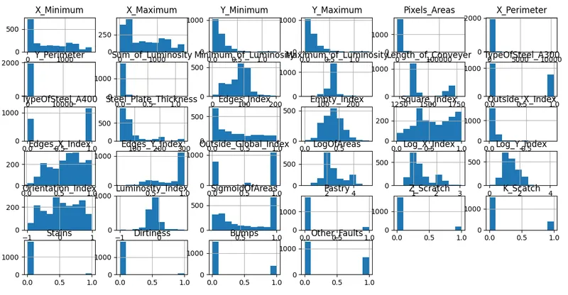
From the above histogram plot we can see that the data is not uniform so standardisation has to be performed on the dataset to derive meaningful results.

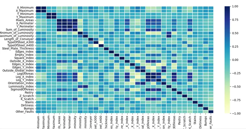
The above correlation matrix shows the co dependence of each factor on one another

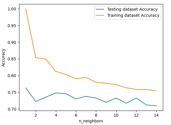
The test and train data accuracy is shown for various k values. The k value for the test dataset is difficult to comprehend as it is not stable. However the training dataset's elbow graph can be seen clearly.

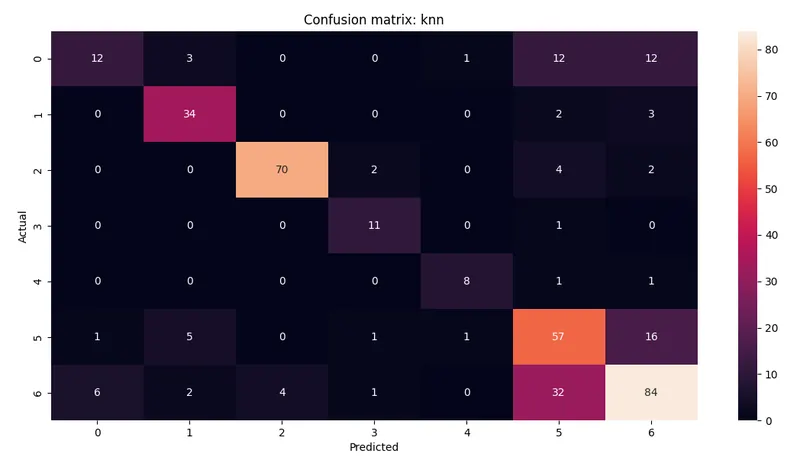
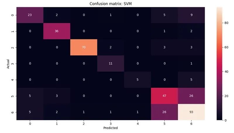
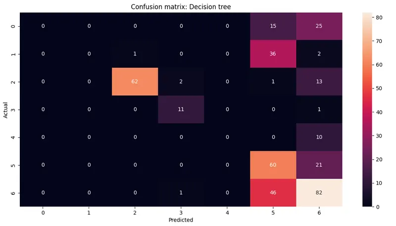
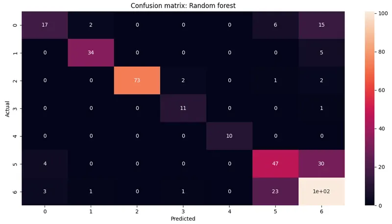
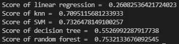
For this particular dataset the accuracy of random forest seems to produce superior results in comparison to the score value of knn.

Why linear regression can't be used to classify data:

There are two things that explain why Linear Regression is not suitable for classification. The first one is that Linear Regression deals with continuous values whereas classification problems mandate discrete values.
The second problem is regarding the shift in threshold value when new data points are added.

Find more information from the below link:
https://medium.com/analytics-vidhya/why-linear-regression-is-not-suitable-for-classification-cd724dd61cb8#:~:text=There%20are%20two%20things%20that,new%20data%20points%20are%20added.

2. Pros and cons of knn

Pros:

1. K-NN is pretty intuitive and simple: K-NN algorithm is very simple to understand and equally easy to implement. To classify the new data point K-NN algorithm reads through whole dataset to find out K nearest neighbors.
2. K-NN has no assumptions: K-NN is a non-parametric algorithm which means there are assumptions to be met to implement K-NN. Parametric models like linear regression has lots of assumptions to be met by data before it can be implemented which is not the case with K-NN.
3. No Training Step: K-NN does not explicitly build any model, it simply tags the new data entry based learning from historical data. New data entry would be tagged with majority class in the nearest neighbor.
4. It constantly evolves: Given it’s an instance-based learning; k-NN is a memory-based approach. The classifier immediately adapts as we collect new training data. It allows the algorithm to respond quickly to changes in the input during real-time use.
5. Very easy to implement for multi-class problem: Most of the classifier algorithms are easy to implement for binary problems and needs effort to implement for multi class whereas K-NN adjust to multi class without any extra efforts.
6. Can be used both for Classification and Regression: One of the biggest advantages of K-NN is that K-NN can be used both for classification and regression problems.
7. One Hyper Parameter: K-NN might take some time while selecting the first hyper parameter but after that rest of the parameters are aligned to it.
8. Variety of distance criteria to be choose from: K-NN algorithm gives user the flexibility to choose distance while building K-NN model.
   1. Euclidean Distance
   2. Hamming Distance
   3. Manhattan Distance
   4. Minkowski Distance

Cons:

1. K-NN slow algorithm: K-NN might be very easy to implement but as dataset grows efficiency or speed of algorithm declines very fast.
2. Curse of Dimensionality: KNN works well with small number of input variables but as the numbers of variables grow K-NN algorithm struggles to predict the output of new data point.
3. K-NN needs homogeneous features: If you decide to build k-NN using a common distance, like Euclidean or Manhattan distances, it is completely necessary that features have the same scale, since absolute differences in features weight the same, i.e., a given distance in feature 1 must means the same for feature 2.
4. Optimal number of neighbors: One of the biggest issues with K-NN is to choose the optimal number of neighbors to be consider while classifying the new data entry.
5. Imbalanced data causes problems: k-NN doesn’t perform well on imbalanced data. If we consider two classes, A and B, and the majority of the training data is labeled as A, then the model will ultimately give a lot of preference to A. This might result in getting the less common class B wrongly classified.
6. Outlier sensitivity: K-NN algorithm is very sensitive to outliers as it simply chose the neighbors based on distance criteria.
7. Missing Value treatment: K-NN inherently has no capability of dealing with missing value problem.