Week 1- Mixing Tee

AIM :

• To set up steady-state simulations to compare the mixing effectiveness when hot inlet temperature is 36⁰C & the Cold inlet is at 19⁰C.
  
  
• The given cases to be studied are-
  • Case 1
  • Short mixing tee with a hot inlet velocity of 3m/s.
  • Momentum ratio of 2, 4.
  • Case 2
  • Long mixing tee with a hot inlet velocity of 3m/s.
  • Momentum ratio of 2, 4.
    Momentum ratio = velocity at cold inlet / velocity at hot inlet
• To use the k-epsilon and k-omega SST model for the first case and based on your judgment use the more suitable model for further cases.
  
  

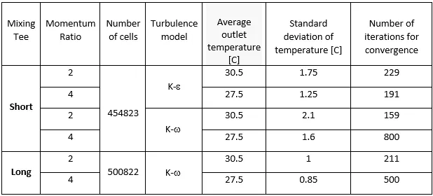
• In a table, compare the following values from the 2 cases.

  1. Cell count
  2. Average outlet temperature
  3. Number of iterations for convergence

• Expected results:

  1. Velocity and temperature contour plots on the cut planes along and across the pipe.
  2. Velocity and temperature line plots along and across the length of the pipe.
  3. Perform Mesh independent study for any one case.
  4. Discuss the effect of length and momentum ratio on results.

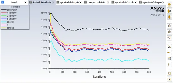
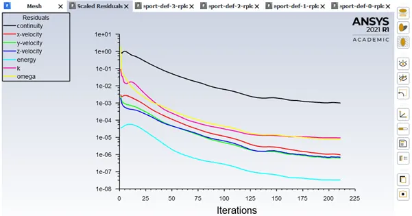
  For each simulation, you need to show the convergence plot

Theory :

`k-epsilon:`

Mathematical representation:

The turbulent energy k is given by:

where U is the mean flow velocity and I is the turbulence intensity.

The turbulence intensity gives the level of turbulence and can be defined as follows:

where u′ is the root-mean-square of the turbulent velocity fluctuations given as:

The mean velocity U can be calculated as follows:

The turbulent dissipation rate can be calculted using the following formula:

where `C_(mu)` is the turbulence model constant which usually takes the value 0.09, k is the turbulent energy, l is the turbulent length scale.

The turbulence length scale describes the size of large energy-containing eddies in a turbulent flow.

The turbulent viscosity `v_t` is, thus, calculated as:

What is `k-epsilon` model –

The k-epsilon (k−ϵ) model for turbulence is the most common to simulate the mean flow characteristics for turbulent flow conditions. It belongs to the Reynolds-averaged Navier Stokes (RANS) family of turbulence models where all the effects of turbulence are modelled.

It is a two-equation model. That means that in addition to the conservation equations, it solves two transport equations (PDEs), which account for the history effects like convection and diffusion of turbulent energy. The two transported variables are turbulent kinetic energy (k), which determines the energy in turbulence, and turbulent dissipation rate (ϵ), which determines the rate of dissipation of turbulent kinetic energy.

The k−ϵ model is shown to be reliable for free-shear flows, such as the ones with relatively small pressure gradients, but might not be the best model for problems involving adverse pressure gradients, large separations, and complex flows with strong curvatures.

Difference between k epsilon and realizable k epsilon

There exist different variations of the k-epsilon model such as Standard, Realizable, RNG, etc. each with certain modifications to perform better under certain conditions of the fluid flow.

The realizable k-ɛ model differs from the standard k−ɛ model in two ways. Firstly, it contains a new formulation for the turbulent viscosity: Cμ is not a constant like in the standard model but a variable The second difference is a new transport equation for the dissipation rate, ɛ, that is derived from an exact equation for the transport of the mean-square vorticity fluctuation.

As a result, it mainly gives improved predictions for the spreading rate of jets, a superior ability to capture the mean flow of complex structures and for flows involving rotation, boundary layers under strong adverse pressure gradients, separation and re circulation. If you predict such flow in your case you should really think about to use this variation of the k-ɛ model.

But both model variants do use wall functions. So, no matter if you use the standard or realizable k−ɛ model you must make sure the y+ -values in your first cell near the wall must not be below 30 and should not excessively exceed values of 100. If your mesh does not fulfil these requirements you need to re mesh your geometry to get reasonable results.

You cannot overcome a poor-quality mesh with changing to another turbulence model, especially not if the other equally uses wall functions.

Velocity values for different momentum ratios:

At inlet x:
Velocity = 3m/s
Temperature = 36 degree centigrade

At inlet y:
Velocity = 6m/s
Temperature = 19 degree centigrade.

How did we arrive at these values of velocity?

Momentum ratio = velocity at cold inlet / velocity at hot inlet
i.e., For a particular value of momentum ratio
Velocity at cold inlet=Momentum ratio*Velocity at hot inlet

If momentum ratio = 2,
Velocity at cold inlet = 2*3
= 6m/s

If momentum ratio = 4,
Velocity at cold inlet = 4*3
= 12m/s

The given equation to calculate the Temperature of the mixture is as given below.

The mass flow rate of air can be given by the following formula:

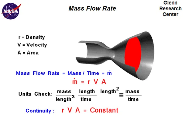
For momentum ratio = 2:

`m_(hot)=rho_(36^0C)*A_(cold)*v_(hot)`

We know that ,
`rho_(hot) = rho_(36^0C) = 1.1427(kg)/m^3, A_(hot) = 897.79mm^2 = 897.79*10^(-6)m^2, v_(hot) = 3m/s`
`rho_(cold) = rho_(19^0C) = 1.2096(kg)/m^3, A_(hot) = 224.84mm^2 = 224.84*10^(-6)m^2, v_(hot) = 6m/s`
So,
`m_(hot) = 1.1427(kg)/m^3*897.79*10^(-6)m^2*3m/s= 3.078*10^(-3)(kg)/s`

`m_(cold)=1.2096(kg)/m^3*224.84*10^(-6)m^2*6m/s= 3.078*10^(-3)(kg)/s`

`T_(mix) = (m_(hot)*T_(hot)+m_(cold)*T_(cold))/( m_(hot)+ m_(cold))`

`T_(mix) = 30.11427^0C`

For momentum ratio = 4:

`m_(hot)=rho_(36^0C)*A_(cold)*v_(hot)`

We know that ,
`rho_(hot) = rho_(36^0C) = 1.1427(kg)/m^3, A_(hot) = 897.79mm^2 = 897.79*10^(-6)m^2, v_(hot) = 3m/s`
`rho_(cold) = rho_(19^0C) = 1.2096(kg)/m^3, A_(hot) = 224.84mm^2 = 224.84*10^(-6)m^2, v_(hot) = 12m/s`
So,
`m_(hot) = 1.1427(kg)/m^3*897.79*10^(-6)m^2*3m/s = 3.078*10^(-3)(kg)/s`

`m_(cold)=1.2096(kg)/m^3*224.84*10^(-6)m^2*12m/s = 3.263*10^(-3)(kg)/s`

`T_(mix) = (m_(hot)*T_(hot)+m_(cold)*T_(cold))/( m_(hot)+ m_(cold))`

`T_(mix) = 27.24^0C`

Mesh independence study :

Momentum ratio: 2

K-`epsi` Model:

Setting up geometry

Geometry:

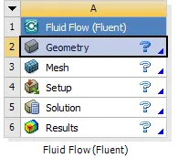
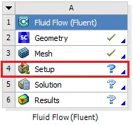
Open fluent and drag the fluent module into the workbench.
Now double click on 'Geometry' to upload geometry.
This operation would allow us to enter the space claim.

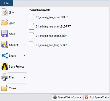
First thing would be to import the test model’s geometry.
To do this go to file in spaceclaim, click on open and select the desired file.

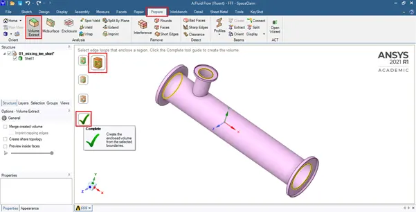
Once you select the file, it appears in the main spaceclaim interface.

The operation we would be performing would be to 'CAD cleanup' the geometry.
We will have to generate a fluid volume to monitor the fluid interaction within the cavity of the CAD model that has been imported.
To create the fluid volume, you will have to go to prepare and then select volume extract.
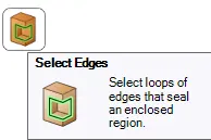
Within the volume extract go to select edges and hit on complete to generate a volume.

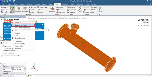
Now hide the CAD model by unchecking the box next to 'Shell1' which is present under structure right click on it and hit supress for physics to exclude it for fluid interactions.

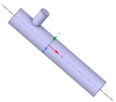
The imported geometry will look as shown above.

Close the spaceclaim window.

Mesh:

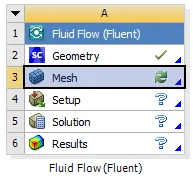
Next would be to open up the fluid volume to mesh.

Geometry Mesh:

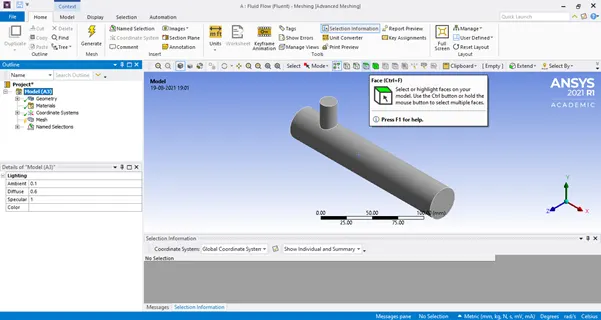
To name the face of the geometry you will have to press N after choosing the side you will be naming.

Below we see how we name the side.

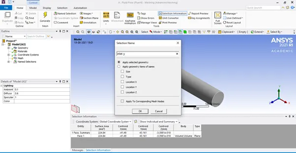
Similarly, we will have to name the ‘inlet x’, ‘walls’ & ‘Outlet’.

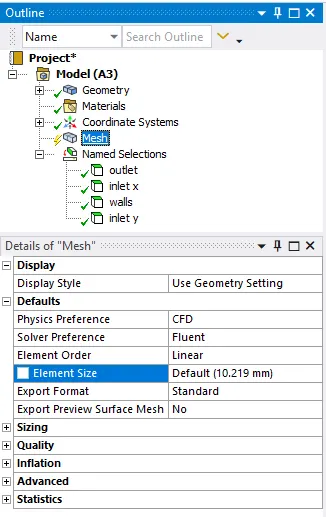
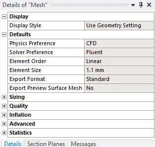
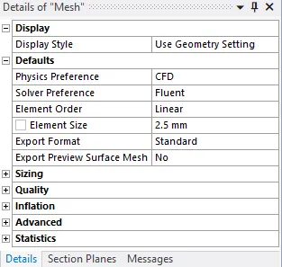
Under Mesh, we will have to select the element size.
Here since having a finer mesh allows us to view the temperature distribution better, we will have to choose the element size as 1.1.
Any other value below 1.1 would result in an error.

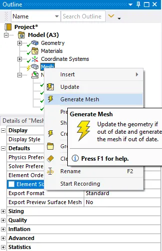
After specifying the element size, we will have to right click on Mesh and select Generate Mesh option.

This allows for us to generate mesh elements for the entire fluid volume.

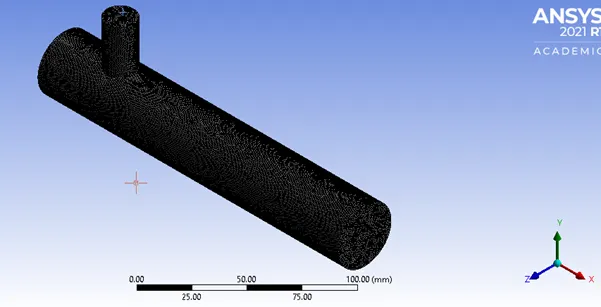
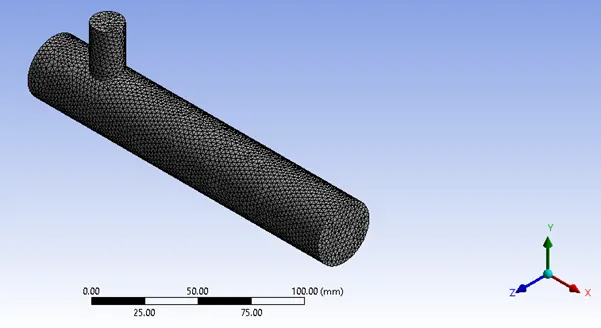
This is the mesh generated for the entire fluid volume.

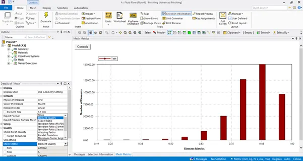
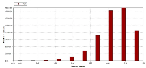
To view the quality of the mesh, go to mesh and search for quality. Under quality you will find Mesh metric now choose Element Quality.

The above Element Quality shows that the quality is good.

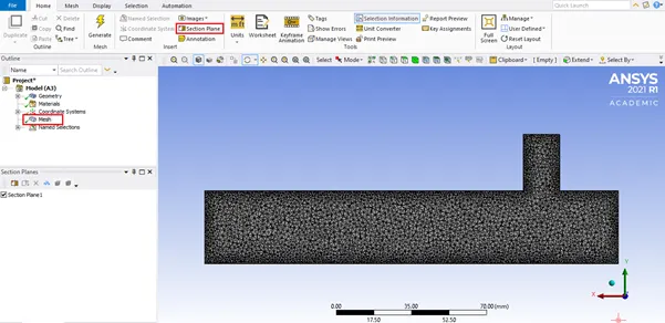
Section view of the geometry.

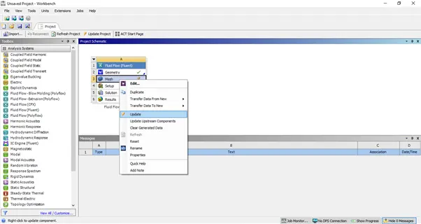
We will have to close the mesh window and open the setup window to solve the transport equations.

Setup:

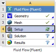
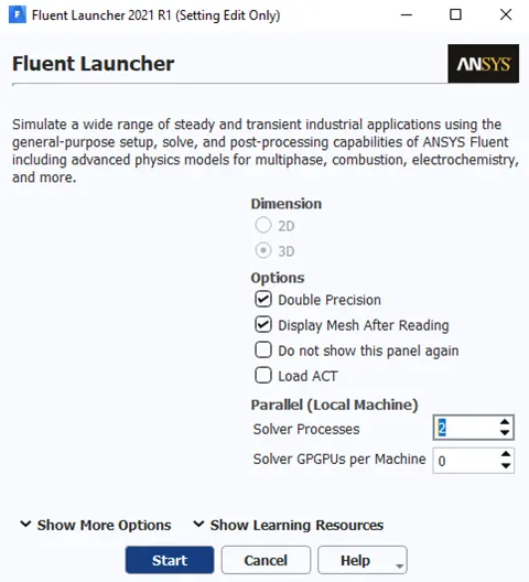
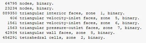
If the specified mesh element size generated 512000 cells then ANSYS student would throw an error.

The correct remedial action would be to reduce the element size.
This can be done by going to mesh again and changing the element size values.

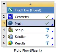
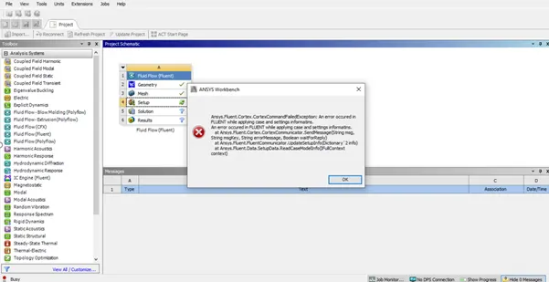
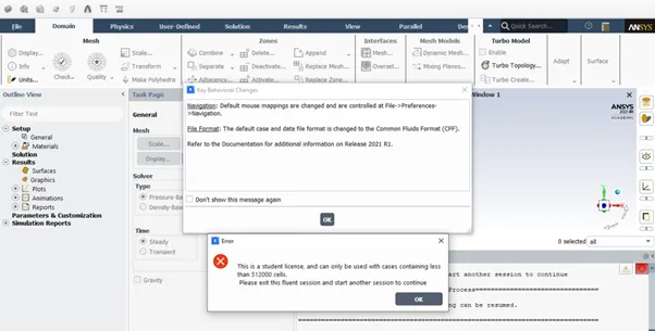
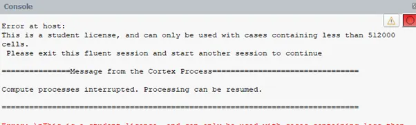
This is how the error messege looks like.

However, for element size of 1.1mm the cells generated is within 512000 limit.

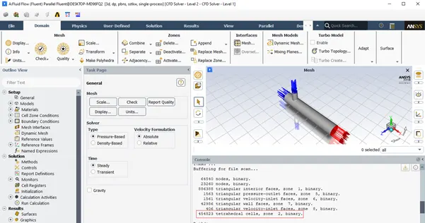
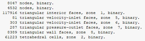
The number of cells is close to 500,000.

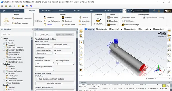
The type of solver we will be using will be a ‘Pressure-based’, ‘Absolute’ and ‘steady’ state simulation.

We will check the ‘energy’ box to ask the solver to solve for energy equation.

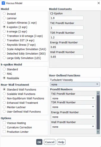
Click on 'viscous' and choose the type of turbulence model.

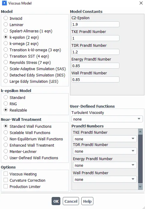
The Viscous Model option allows us to choose the type of simulation.

In this exercise, realisable K-epsilon model will be chosen.

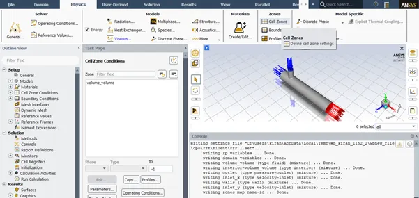
Next, select the Cell zone condition & hit on volume_volume and then hit on edit it if the fluid used in the system needs to be changed.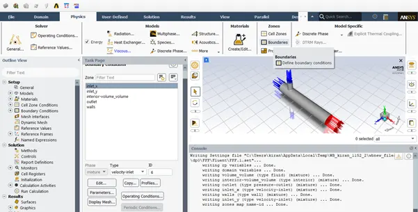

Next would be to setup the boundaries for the inlets & outlet.

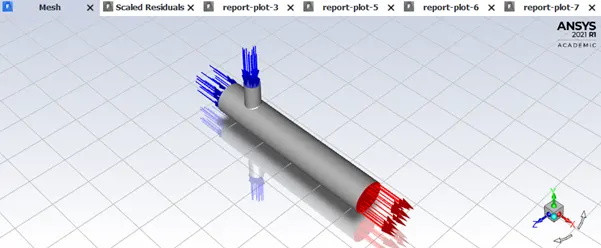
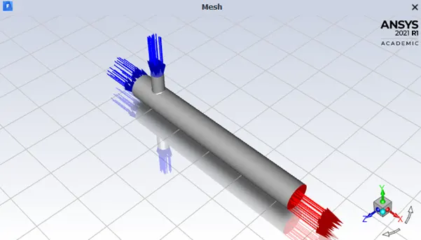
This step allows us to input velocity boundary conditions at each and every inlet, it is interesting to note that Fluent chooses an appropriate boundary condition based on the user defined names of the inlets.

Going by the momentum ratio we can specify the inlet velocities for the hot and cold fluids.
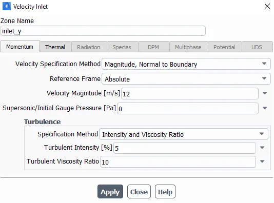
The ‘inlet x’ being the inlet through hot air comes in must be given an inlet velocity 3m/s as specified in the question, whereas the cold inlet (inlet y) fluid velocity must be given an inlet velocity of 6m/s.

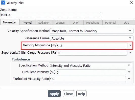
This is the window we get to see once we select an inlet and then hit edit.
The temperature of the inlet fluid can also be changed by clicking thermal on the popup window.
The temperature and velocity values for each inlet is given below.
At inlet x:
Velocity = 3m/s
Temperature = 36 degree centigrade

At inlet y:
Velocity = 6m/s
Temperature = 19 degree centigrade.

How did we arrive at these values of velocity?

Momentum ratio = velocity at cold inlet / velocity at hot inlet
i.e., For a particular value of momentum ratio
Velocity at cold inlet=Momentum ratio*Velocity at hot inlet

If momentum ratio = 2,
Velocity at cold inlet = 2*3
= 6m/s

If momentum ratio = 4,
Velocity at cold inlet = 4*3
= 12m/s

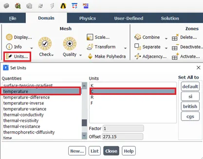
By clicking on ‘units’ we can view the temperature in a desirable unit.

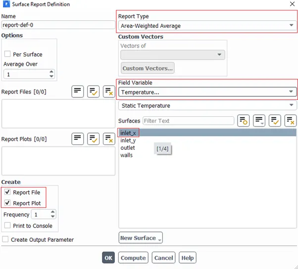
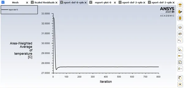
To monitor some physical quantities for example, at the outlet if you want to watch the temperature
Click on definitions, then go to New, after this click on surface report and then area weighted average.

The boxes in red signify changes to the original settings
The changes are as follows,
The report type is Area-weighted average.
Field variable we are interested in monitoring will be – Velocity & Temperature.
To obtain report file & report plot we will have to check the boxes
We must choose a surface over which we need the area weighted average of a specific parameter.

To manage the reports generated go to definitions, then click edit.

Area weighted average:

Area-weighted average: You can find the average value on a solid surface, such as the average heat flux on a heated wall with a specified temperature.

The area-weighted average of a quantity is computed by dividing the summation of the product of the selected field variable and facet area by the total area of the surface:

`1/AintphidA=1/A*sum_(i=1)^nphi_i|A_i|`

Standard deviation:

You can find the standard deviation of a specified field variable on a surface, such as enthalpy, viscosity, and velocity.

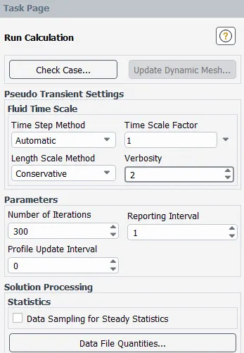
After this step click on initialise under solutions.

Double click on run calculation, to to calculate and generate required reports.
The number of iterations that has been mentioned, here 300 iterations.

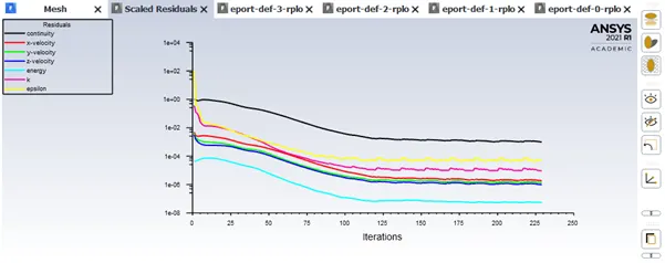
Console:

Even though the number of iterations specified is 300, the graphs clearly show iterations lesser than 229.

Plots:

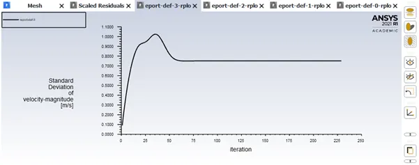
Standard deviation of velocity: 0.75m/s

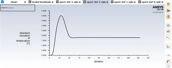
Standard deviation of temperature: 1.75C

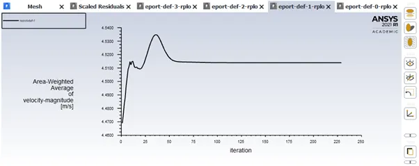
Average velocity: 4.51m/s

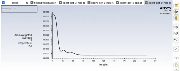
Average temperature: 30.5C

Results:

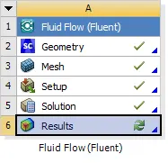
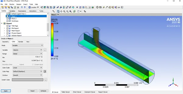
Now open the results window to see the contours of variables.

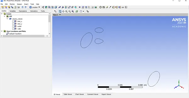
The initial display on the screen would be as seen above.

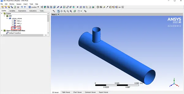
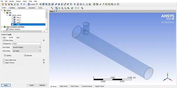
When you check the 'walls' box under 'volume_volume' an envalope of the wall is generated.

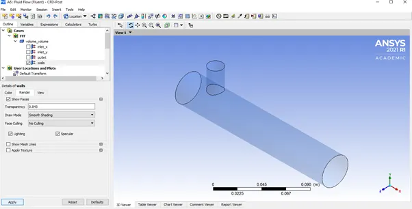
To be able to see the contours within the volume we need transparency so, to increase transparency double click on walls then go to 'Render' under 'Details of walls'. Here increase the transparency to a comfortable level of your desired choice.

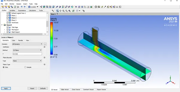
To look at velocity distribution & the pressure distribution to see if it makes sense.
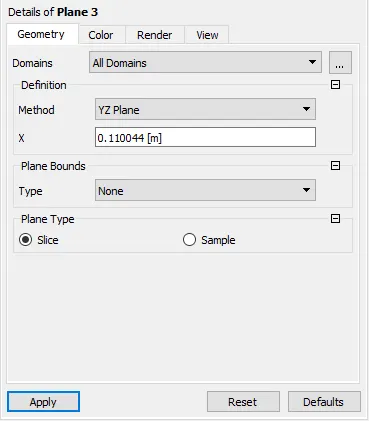
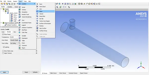
In post processing window: Go to, Insert then go to, Plane.
Now you get to name the plane then click OK
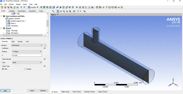
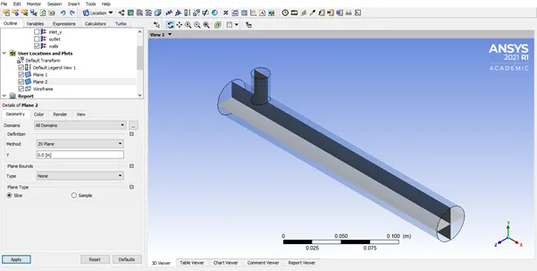
Choose the plane XY for a plane to appear in the following fashion.
If we click Apply, then this plane appears in the middle of the geometry.

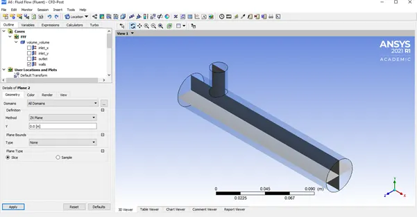
Choose the plane XZ for a plane to appear in the following fashion.
If we click Apply, then this plane appears in the middle of the geometry.

After creating the 2 orthogonal planes we will have to color the planes to see the velocity and temperature distribution.

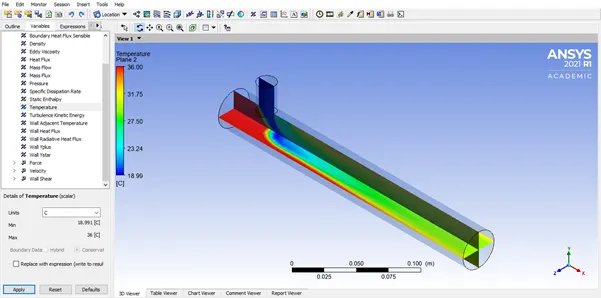
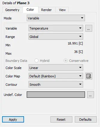
To color the plane accordingly, double click on the plane you wish to see the color on and then go to color tab under the details of the plane now change the mode to variable and select temperature or velocity from the variable dropdown window. Click apply to see changes.

To change units to Celsius from kelvin scale, click on the things enclosed in red boxes.

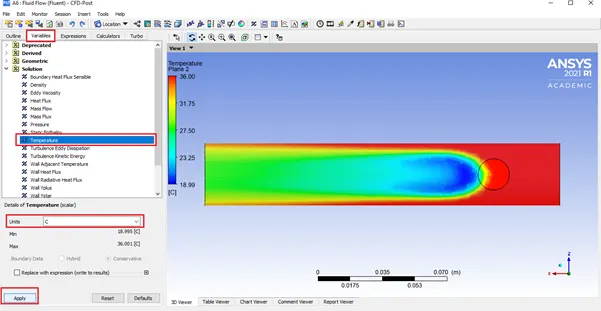
Go to variables, double click on 'Temperature' change 'units' to desired unit.

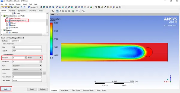
To modify the legend, double click on 'Default legend view' go to 'Precision' and change it to a value of '2'.
Now, to change the scale of the legend click on the drop down box next to 'Precision'.

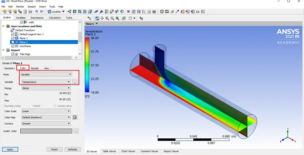
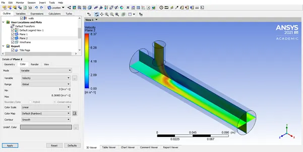
To color the planes with a variable that needs to be observed, double click on a particular plane then go to 'Details of plane' and change mode to 'variable'.
Now, change variable which needs to be observed.

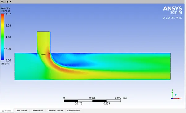
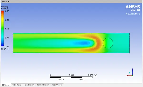
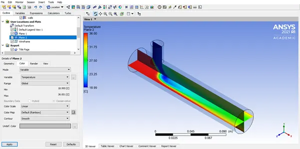
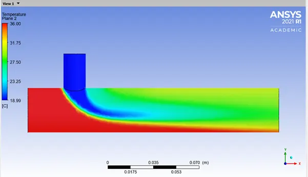
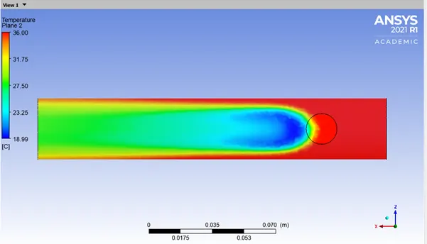
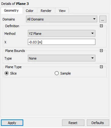
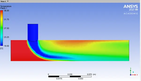
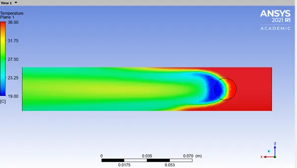
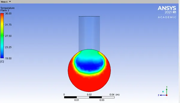
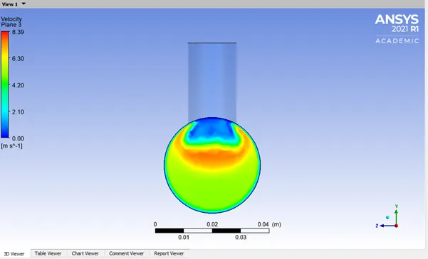
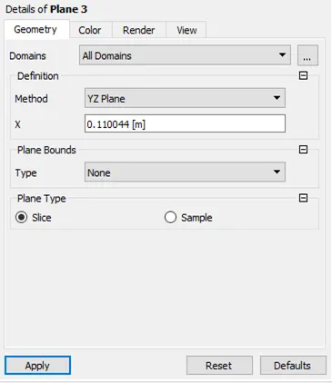
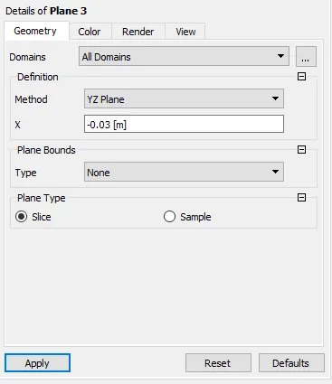
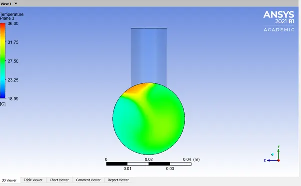
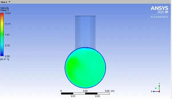
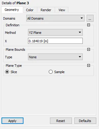
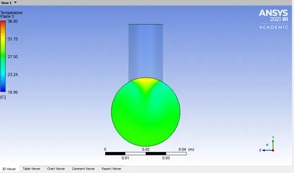
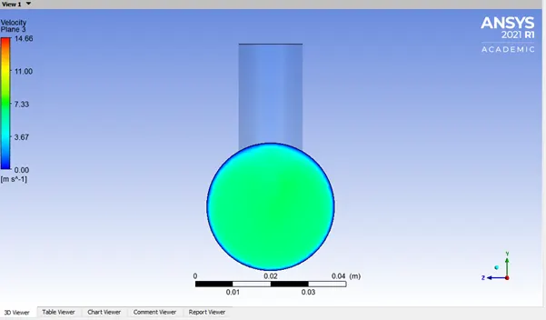
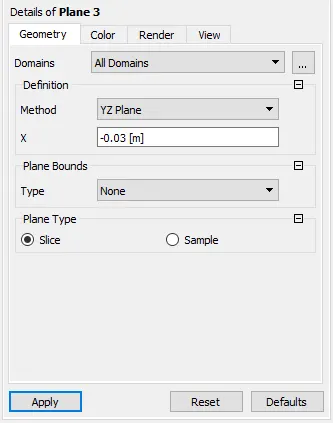
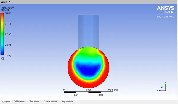
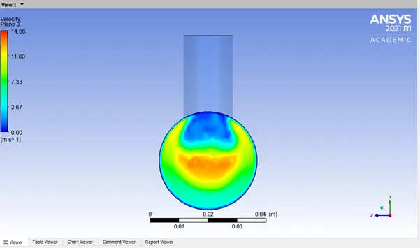
X distance is chosen to be -0.03m because it is the distance just at the point of mixing in the Mixing-Tee(At the junction of 'inlet x' & 'inlet y').
Here we can observe the way fluids of different thermal properties mixes together right after the T-joint.

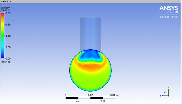
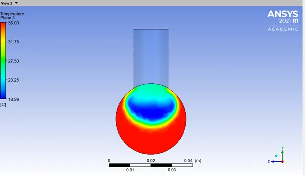
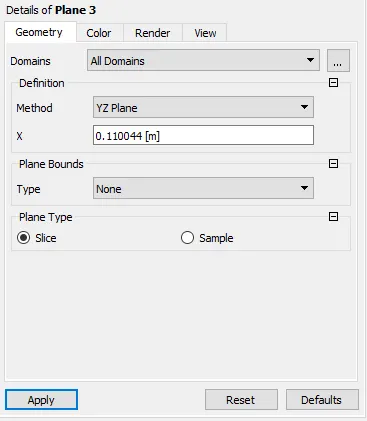
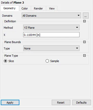
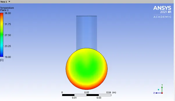
X distance is chosen to be 0.11m because it is the distance just at the end of the Mixing-Tee .
Here we can observe the way fluids of different thermal properties have mixed just before exited the Mixing-Tee .

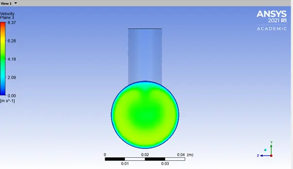
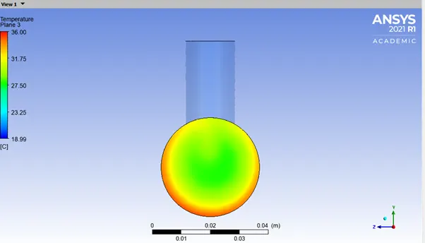
• For element size 2.5mm

Console:

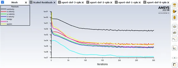
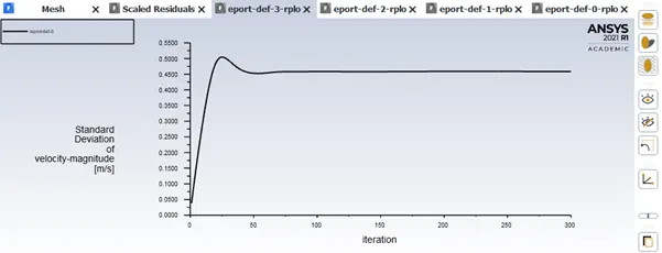
Standard deviation of Velocity = 0.45 m/s

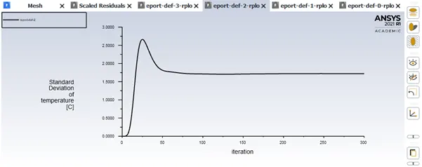
Standard deviation of Temperature = 1.75 degree Celsius

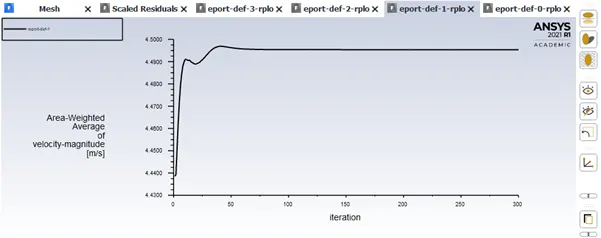
Average velocity = 4.495 m/s

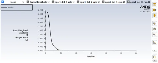
Average Temperature = 30.25 degree Celsius

• For element size 5mm:

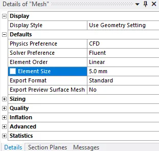
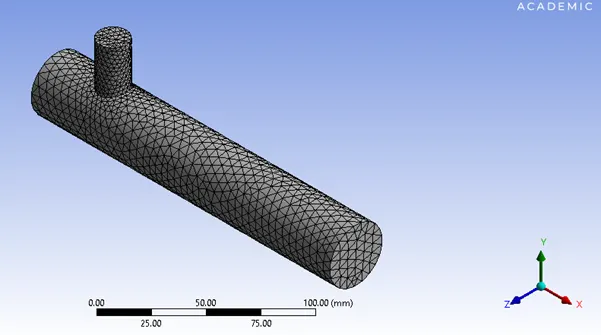
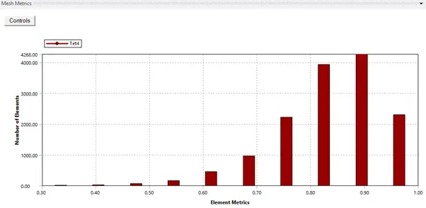
Console:

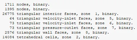
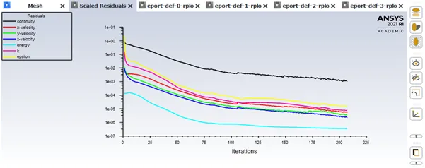
Even though the number of iterations specified is 300, the graphs clearly show iterations lesser than 207.

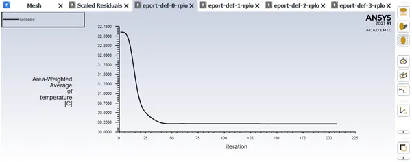
Average temperature = 30.25 degree Celsius

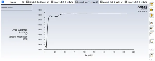
Average velocity = 4.505 m/s

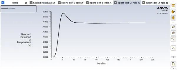
Standard deviation of Temperature = 1.75 degree Celsius

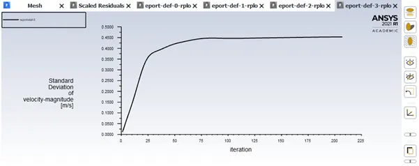
Standard deviation of Velocity = 0.45 m/s

We know that,

If momentum ratio = 2,
Velocity at cold inlet = 2*3
= 6m/s

If momentum ratio = 4,
Velocity at cold inlet = 4*3
= 12m/s

Analytical data:
For momentum ratio =2:
`T_(mix) = 30.11427^0C`
For momentum ratio =4:
`T_(mix) = 27.24^0C`

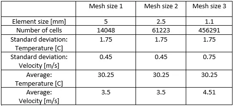
Note that the average temperature at the outlet is found out to be 30.11427C in case 1 when momentum ratio is 2, also the average temperature at the outlet is found out to be 27.24C when momentum ratio is 4.

So, the values we obtained numerically is close to the analytical result.
The only parameter that shows a bit of a variation is the Average velocity, for element size 1.1mm the value of average velocity is different than the velocity values we got from element size 5 & 2.5

Since we are interested in looking at the fluid interaction within the confines of the geometry we will be considering the finest mesh element size configuration.
The smaller the mesh element size the smoother are the contours of variables(Temperature & Velocity).

Momentum ratio: 4

`K-epsilon`:

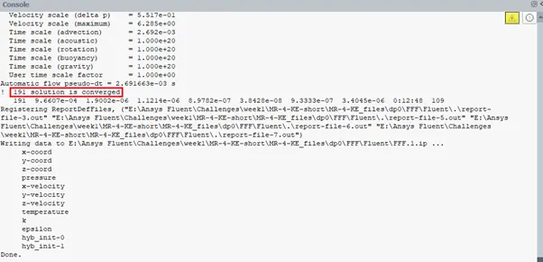
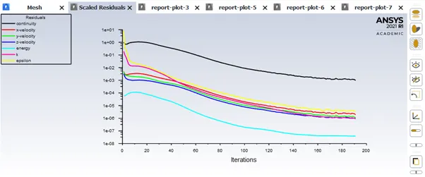
By modifying the case study for 'Element size' 1.1mm, the initial settings remain same but the changes must be changed only in the 'setup' module of the workbench.
Necessary changes have been recorded below.

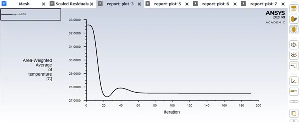
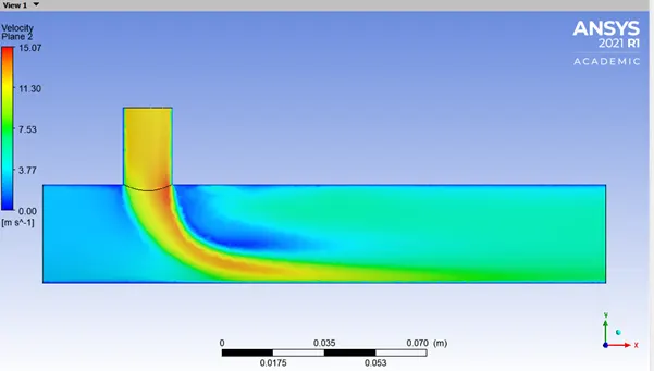
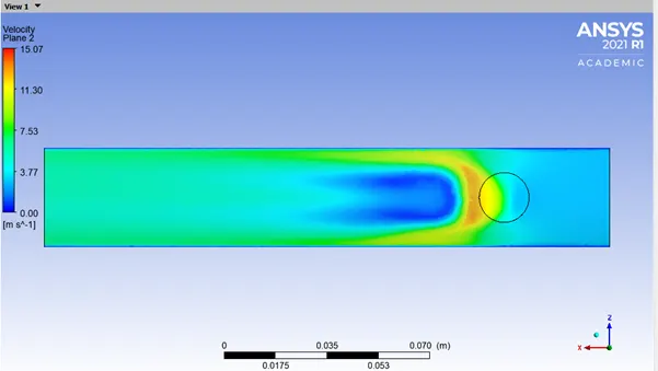
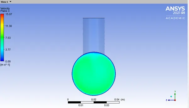
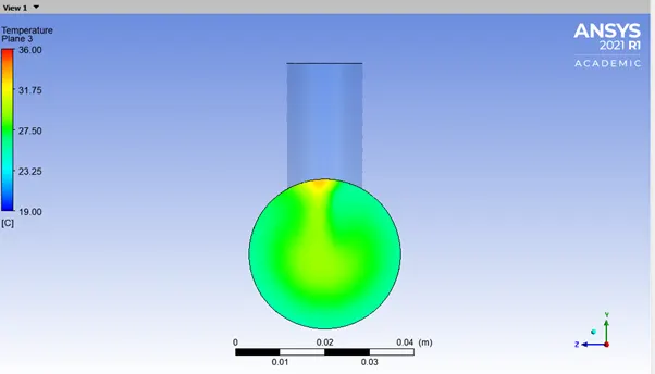
Average temperature = 27.5C

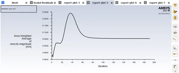
Average velocity = 6.05m/s.

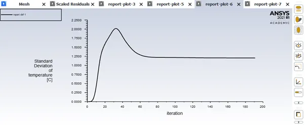
Standard deviation of temperature = 1.25C

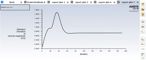
Standard deviation of velocity = 0.7m/s

Results:

Temperature:

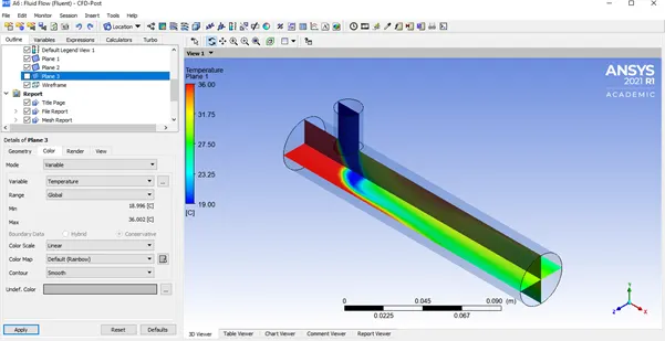
Velocity:

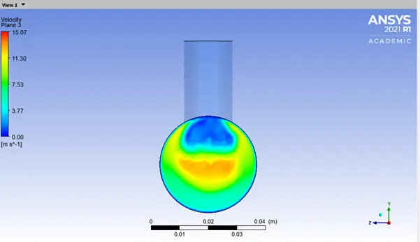
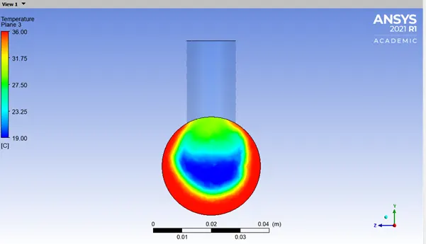
Momentum ratio: 2

`K-omega:`

The k-omega (k−ω) turbulence model is one of the most commonly used models to capture the effect of turbulent flow conditions. It belongs to the Reynolds-averaged Navier-Stokes (RANS) family of turbulence models where all the effects of turbulence are modelled.

It is a two-equation model. That means in addition to the conservation equations, it solves two transport equations (PDEs), which account for the history effects like convection and diffusion of turbulent energy. The two transported variables are turbulent kinetic energy (k), which determines the energy in turbulence, and specific turbulent dissipation rate (ω), which determines the rate of dissipation per unit turbulent kinetic energy. ω is also referred to as the scale of turbulence.

The standard k−ω model is a low Re model, i.e., it can be used for flows with low Reynolds number where the boundary layer is relatively thick and the viscous sublayer can be resolved.

Thus, the standard k−ω model is best used for near-wall treatment. Other advantages include a superior performance for complex boundary layer flows under adverse pressure gradients and separations (e.g., external aerodynamics and turbomachinery). On the contrary, this model has also shown to predict excessive and early separations.

There exist different variations of the k-omega model such as standard k-omega (discussed above), baseline k-omega, k-omega SST, etc., each with certain modifications to perform better under certain conditions of the fluid flow.

Understanding `K-omega` SST

SST stands for shear stress transport. The SST formulation switches to a `k-epsi` behaviour in the free-stream, which avoids the k−ω problem of being sensitive to the inlet free-stream turbulence properties.

The k−ω SST model provides a better prediction of flow separation than most RANS models and also accounts for its good behaviour in adverse pressure gradients. It has the ability to account for the transport of the principal shear stress in adverse pressure gradient boundary layers. It is the most commonly used model in the industry given its high accuracy to expense ratio.

On the negative side, the SST model produces some large turbulence levels in regions with large normal strain, like stagnation regions and regions with strong acceleration. This effect is much less pronounced than with a normal k-epsilon model though.

Difference between K-Epsilon and K-Omega model:

k- epsilon model predicts well far from the boundaries (wall) and k- omega model predicts well near wall. Even though it depends on Y+. We also have SST model which is a combination of these.

Momentum ratio: 2

`K-omega:`

By modifying the case study for 'Element size' 1.1mm, the initial settings remain same but the changes must be changed only in the 'setup' module of the workbench.
Necessary changes have been recorded below.

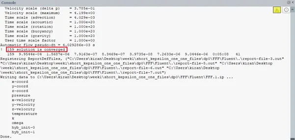
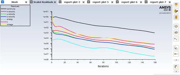
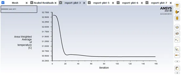
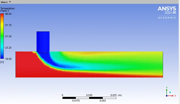
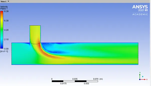
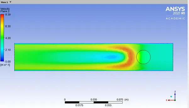
Average temperature = 30.5C

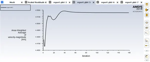
Average veocity = 4.51m/s

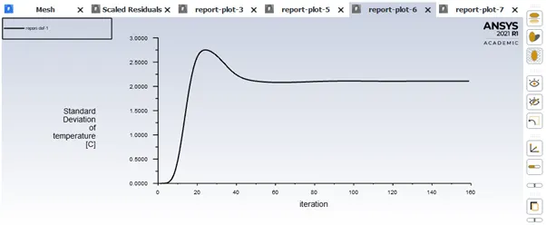
Standard deviation of temperature = 2C

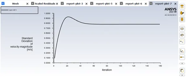
Standard deviation of velocity = 0.8m/s

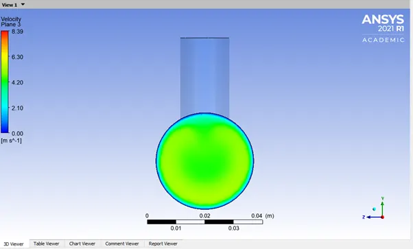
Results:

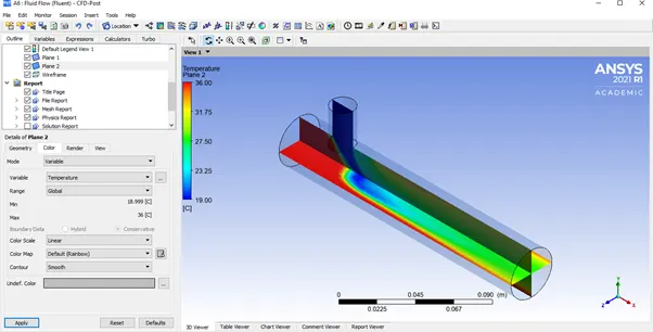
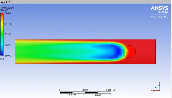
Temperature:

Velocity:

Momentum ratio: 4

`k-omega:`

By modifying the case study for 'Element size' 1.1mm, the initial settings remain same but the changes must be changed only in the 'setup' module of the workbench.
Necessary changes have been recorded below.

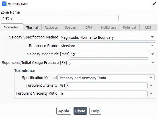
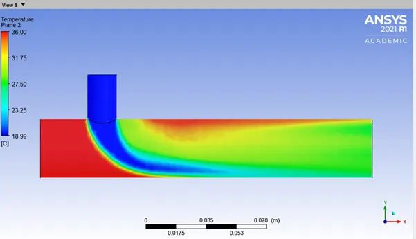
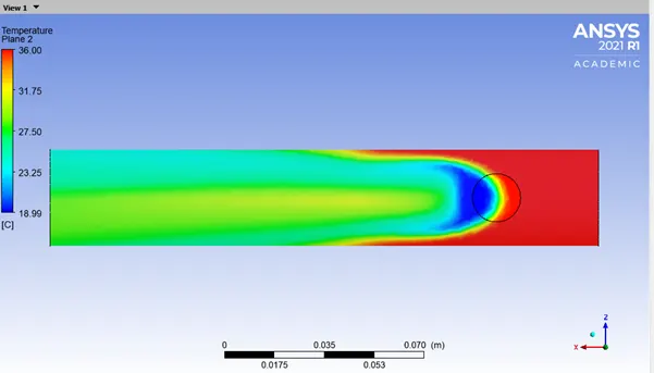
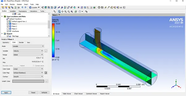
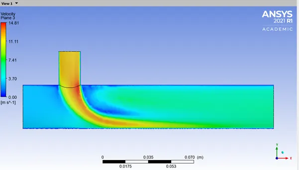
Average temperature = 27.5C

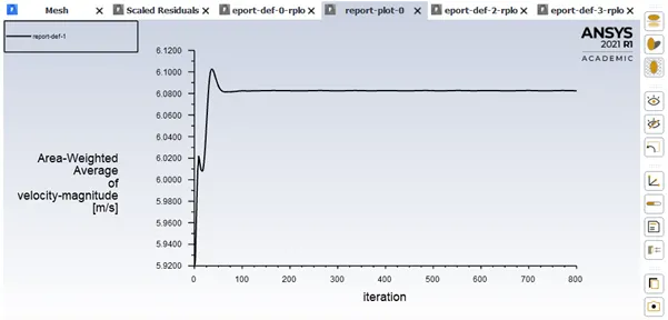
Average velocity = 6.08m/s

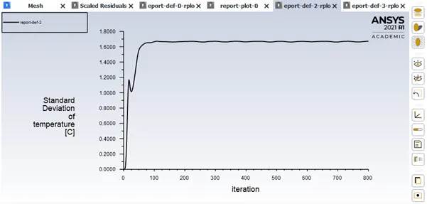
Standard deviation of temperature = 1.6C

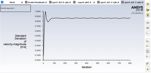
Standard deviation of velocity = 0.85m/s

Results:

Temperature:

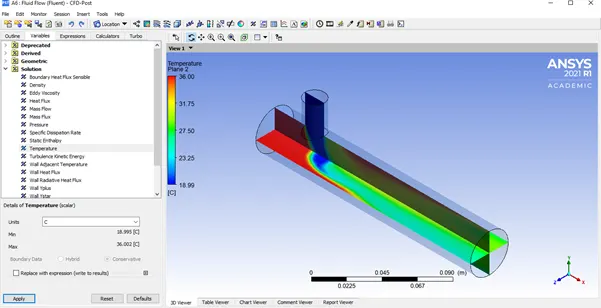
Velocity:

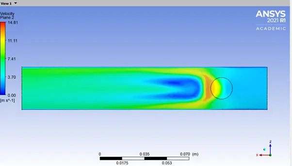
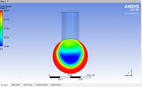
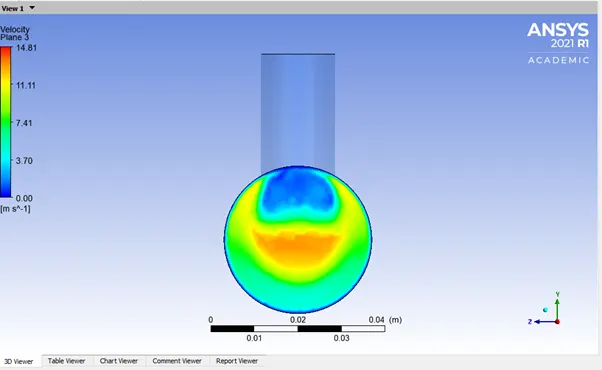
`K-epsi` vs `K-omega` comparison:

The k−ω SST model provides a better prediction of flow separation than most RANS models and also accounts for its good behaviour in adverse pressure gradients. It has the ability to account for the transport of the principal shear stress in adverse pressure gradient boundary layers. It is the most commonly used model in the industry given its high accuracy to expense ratio.

On the negative side, the SST model produces some large turbulence levels in regions with large normal strain, like stagnation regions and regions with strong acceleration. This effect is much less pronounced than with a normal k-epsilon model though.

A stagnation point is a point in a flow field where the local velocity of the fluid is zero.

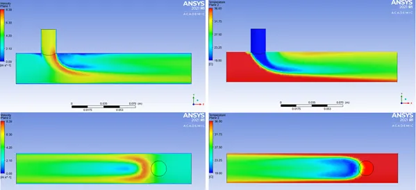
The model used here is a mixing Tee which doesn’t have any fluid medium colliding head on with the model, hence we consider `K-omega` SST as a superior option to consider for our analysis.

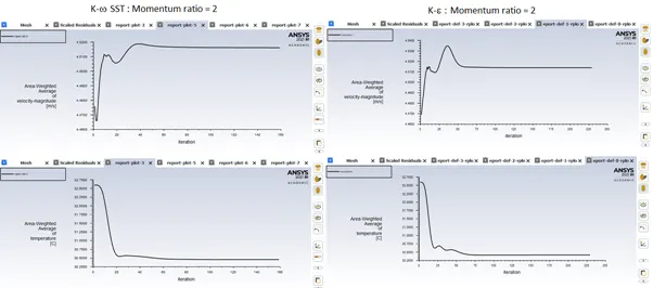
`K-omega` SST Momentum ratio = 2

`K-epsi` Momentum ratio = 2

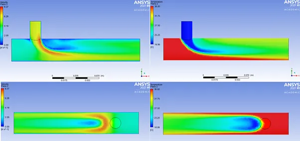
From the above comparison we can see that the contours are well defined in `K-omega` SST model.

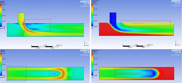
`K-omega` SST Momentum ratio = 2

Parts that have been enclosed within the red box shows significant change in color pattern when compared with the `K-epsi`contour plots.
The differences are significantly visible in the temperature contours.

`K-omega` SST Momentum ratio = 2

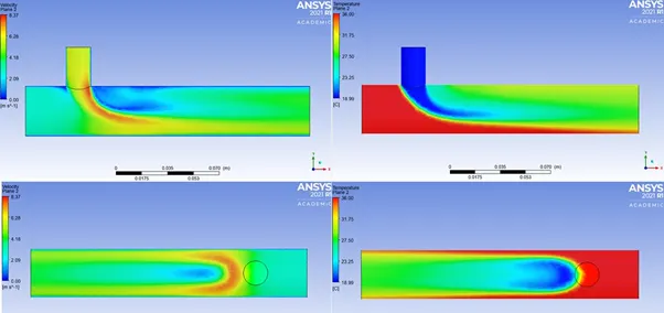
For momentum ratio: 4, short pipe configuration.

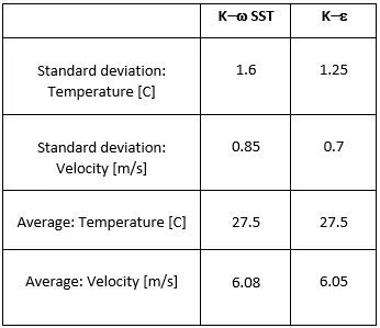
It is always good to have low standard deviation values for any variable that is being observed.

Now it is proven that, using K-`omega` SST turbulence model will be the best choice for Long pipe turbulence simulation.

Long Mixing Tee - Momentum ratio 2:

K-`omega` SST model:

The steps involved in this exercise is similar to the methods used above, hence only the most important changes and it's consequence as a result has been documented here.

Geometry:

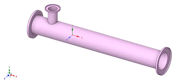
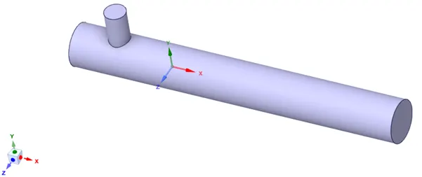
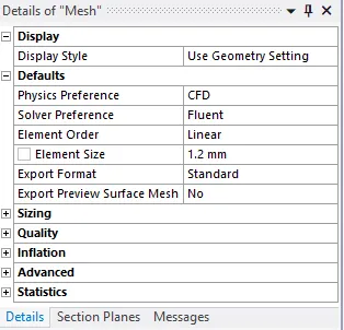
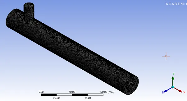
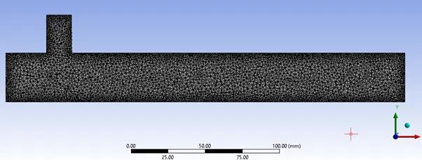
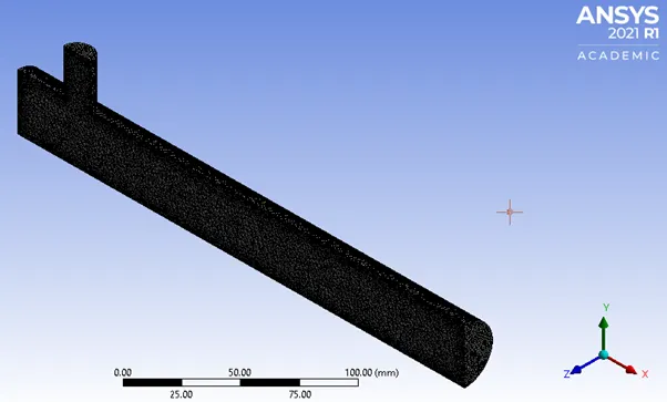
The minimum element size has been found out to be 1.2mm after much trial and error.
Any other value below this value would throw an error.

Setup:

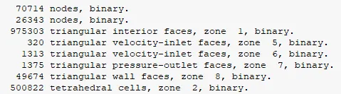
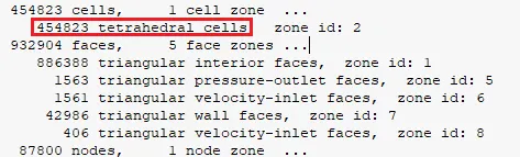
The number of tertahedral cells for this configuration will show up on 'console'.

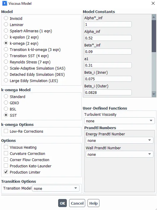
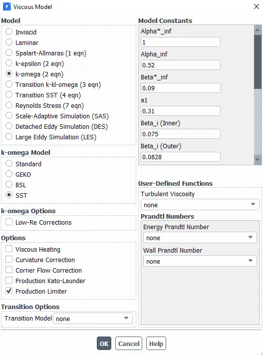
The turbulence model and its configuration can be modified by clicking on 'viscous model'.

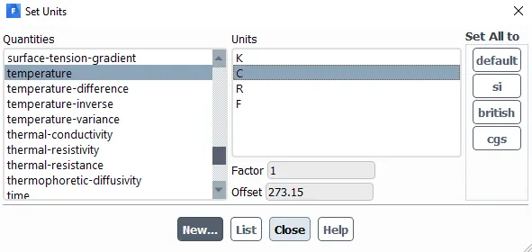
The units of temperature can be changed as shown above.

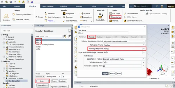
The boundary values can be changed by clicking on the options enclosed in the boxes.

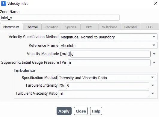
For momentum ratio 2, the magnitude of velocity has been specified.

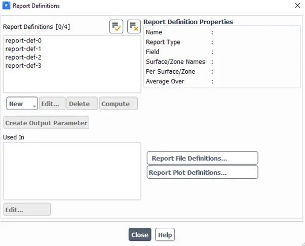
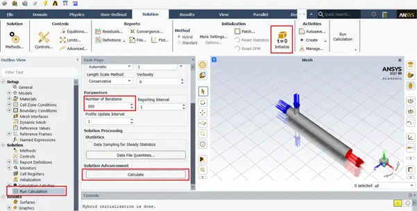
Before proceeding to generate the report, the solution must first be initialised and later the number of iteration limit must be specied under 'Run calculation'.

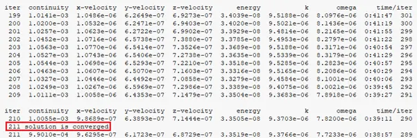
Even though the number of iterations soecified is 500, the solution has converged at 211 iterations.

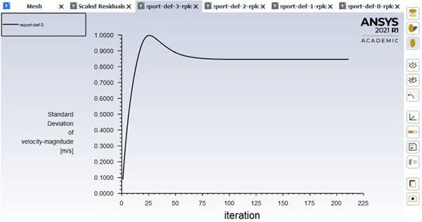
Standard deviation of velocity = 0.85m/s

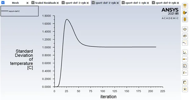
Standard deviation of temperature = 1C

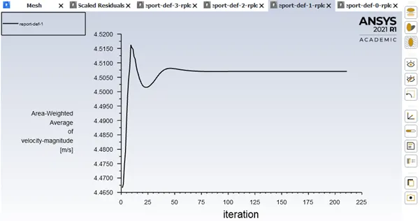
Average velocity = 4.5m/s

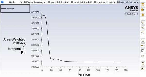
Average temperature = 30.5C

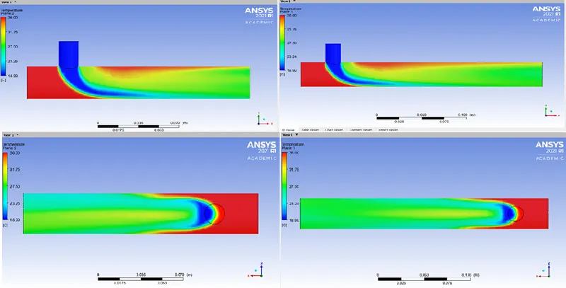
Results:

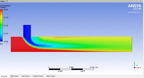
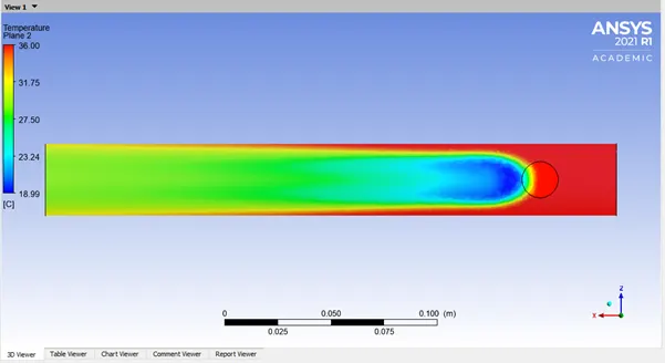
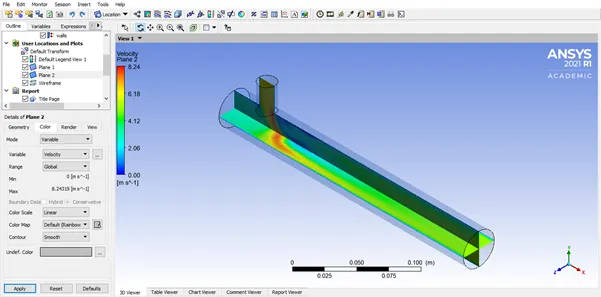
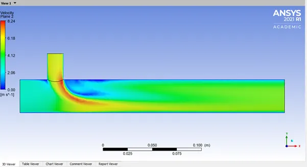
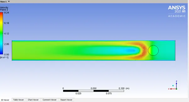
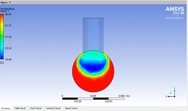
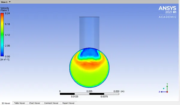
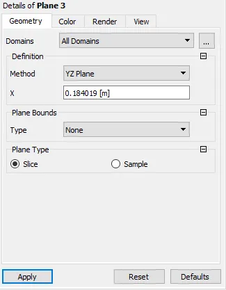
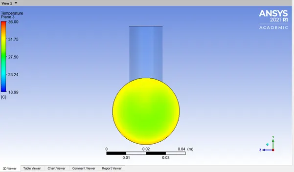
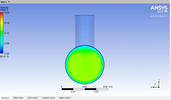
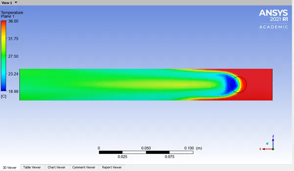
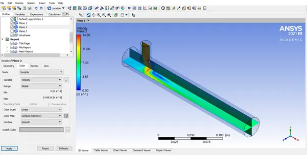
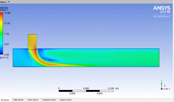
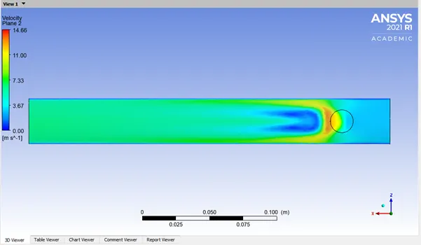
Long Mixing Tee - Momentum ratio 4:

K-`omega` SST model:

Until 'setup' the steps required for this case is same as the ones used above.
Below shown are the changes that must be made to setup and results section in the fluent workbench.

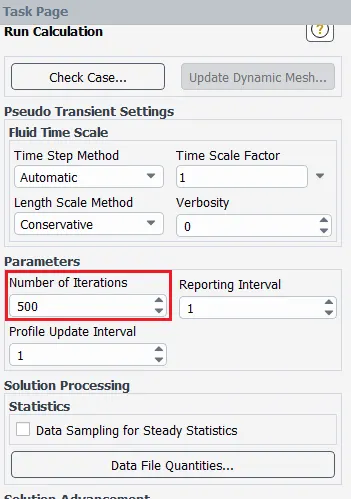
500 iterations has been considered.

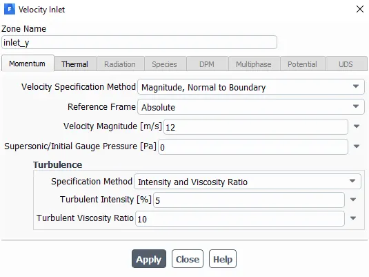
The 'inlet y' velocity value has been changed according to the momentum ratio.

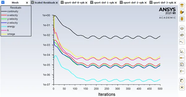
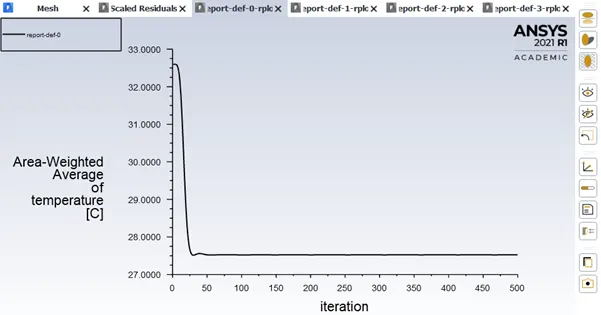
Average temperature = 27.5C

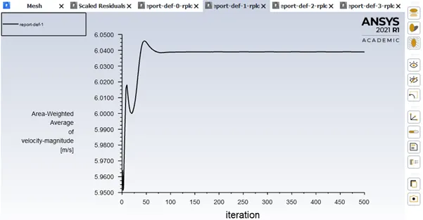
Average velocity = 6.04m/s

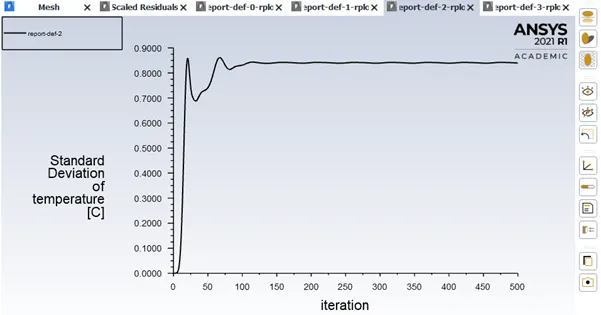
Standard deviation of temperature = 0.8C

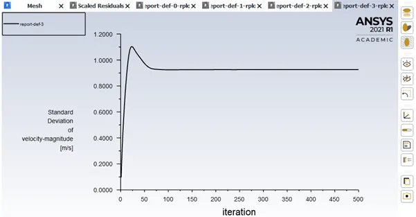
Standard deviation of velocity = 0.95m/s

Results:

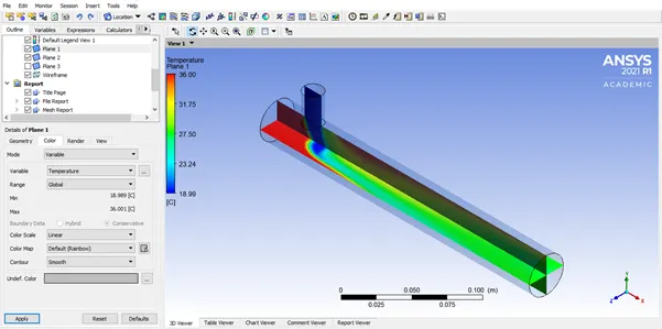
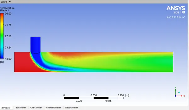
Conclusion:

1. K-omega model is prefered over K-epsilon model because K-omega model can predict well near boundaries of the geometry.
2. The difference between the long and short configuration of the geometry is that the number of iterations required to arrive at the soultion is more in the long mixing tee.
3. The only advantage of having a long mixing tee is that it allows for better mixing of the hot and cold fluid mediums.
   There is not much difference when it comes to end temperatures at the outlet.
4. There is significant difference in the temperature values at the outlet when the results of momentum ratios 2 & 4 are compared.

Reference:

Ansys documentation:
https://d.shikey.com/down/Ansys.Products.2020.R1.x64/install_docs/Ansys.Products.PDF.Docs.2020R1/readme.html

K epsilon :
https://www.cfd-online.com/Wiki/K-epsilon_models
https://en.wikipedia.org/wiki/K-epsilon_turbulence_model
Realisable
https://www.cfd-online.com/Wiki/Realisable_k-epsilon_model

For computing surface integrals :
https://www.afs.enea.it/project/neptunius/docs/fluent/html/th/node416.htm
https://www.afs.enea.it/project/neptunius/docs/fluent/html/th/node415.htm

K-Omega
https://www.cfd-online.com/Wiki/K-omega_models
Equations
https://turbmodels.larc.nasa.gov/sst.html
SST
https://www.cfd-online.com/Wiki/SST_k-omega_model