Week 7 - Auto ignition using Cantera

Objective :

To understand the usage of reactor and reactor network by solving for a set of Methane combustion reactions at different given conditions .

1. Auto Ignition Time for Methane under the following conditions, (simulation time = 10 secs)

• Plot the variation of Auto Ignition time of Methane with a constant temperature of 1250K and pressure varying from 1 to 5 atm.
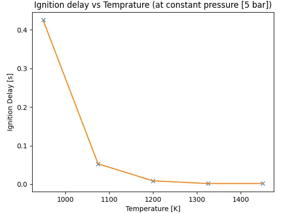
• Plot the variation of Auto Ignition time of Methane with a constant pressure of 5 atm and temperature varying from 950K to 1450K.

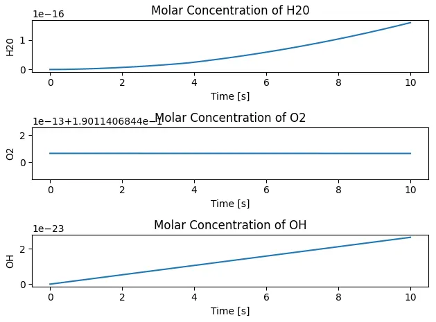
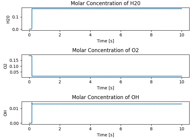
2. Observe and print the rate of change of molar concentrations of the given elements "H2O, O2, OH" with respect to the time, (simulation time = 10 secs)

Explain the behavior of the graph for 2 cases,

• When Temperature is 1000K and pressure 5 bar
• When Temperature is 500K and pressure 5 bar

Auto-ignition temperature :

In the context of a combustible fuel mixture, the auto-ignition temperature is the lowest temperature at which the fuel will spontaneously ignite in a normal atmosphere without an external source of ignition such as a flame or spark.

This temperature is sometimes referred to as the kindling point of the fuel. Raising the temperature of a fuel to its auto-ignition point provides the energy required to initiate the chemical reaction needed for combustion. The auto-ignition temperature for a given fuel decreases as the pressure increases or as the oxygen concentration increases.

Reactor :

Cantera is based purely on Object oriented program (OOP) ,this not only contains objects like 'gas()' OOP also contains Reactor object.

Cantera is simplest reacting system that you can create within the reactor ,there are no gradients,composition & any other thermodynamic properties ie., within the reactor we can assume only 1 value for Pressure & Temprature & composition for any species within the reactor (no spacial gradients)

Each reactor is given a certain volume .

Types of reactors :

• Standard reactor
• Constant pressure reactor
• Ideal gas reactor
• Ideal gas constant pressure reactor

Each reactor has it's own governing equation [depending on whether the system is a closed system or an open system and how heat loss and mass transfer happens]

Reactor Network :

The other object that is important with respect to 0D & 1D calculations is the reactor network.

The reactor just defines the governing equations to be solved . The actual solving part is done by the reactor network .

Ex: Time integration part & ODE part will be solved by using Reactor network .

Even id=f we have one single reactor we need a reactor network & cantera is made in such a way that wihtout reactor network we won't be able to solve the problem.

Once we have a 'Reactor network' object that object will have an 'advance' 'method' .This is going to integrate your system , this in essence allows the reactor to take the second time step .

When 'advance' 'method is called the reactor state changes .

Visual representation :

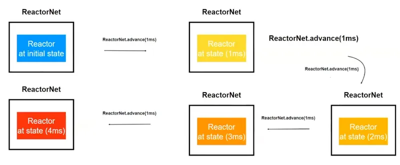
More information on Reactor and Reactor Networks

https://cantera.org/science/reactors.html

Code 1 :

To plot for the variation of Auto Ignition time of Methane with a constant temperature of 1250K and pressure varying from 1 to 5 atm.

Briefing :

The below stated logic applies to Part 1 of the question .

• First we create a gas object where 'ct' is the module ,Solution is a class & this solution class is used to create an instance of the 'object' called 'gas' .
• Next we set us Temprature ,Pressure & concentration & we can call these as the attributes for 'gas' object .
• Each value of temperature or pressure runs through the for loop to create a unique gas object which in turn creates a new value for 'r'
• If we type 'help(r)' ,we will see all the required details for setting up of a reactor like details about the Methods & etc.,
• We now proceed to create a reactor net ,the basic flow of code must always start with creation of an instance object of reactor network & then pass the assigned reactor to it.
• We set the initial time as 0 for us to start the time step at 0 seconds.
• A solution array for the gas object is created & we also pass the time values to it ,the solution array describes the state of the reactor object . At each time step the reactor array assumes new set of values .An interesting feature of Reactor array is that it contains data about Temperature ,Pressure & etc.,
• Now we start another 'for' loop to run each pressure value for 10 seconds with an increment in time step of 1e-3 & we append the atate of the reactor at the end of time 1e-3 at that iteration for a particular value of 'n'.
  States of reactors contain all the data of temprature , pressure , concentration & etc.,
• The if loop works by saving the time taken for the fuel to reach auto ignition temterature ,essentially what we will know by doing this is the ignition delay.
• Now with all the data that we want we can plot it appropriately .

import numpy as np
import cantera as ct 
import matplotlib.pyplot as plt

gas=ct.Solution('gri30.xml')
T=1250
P_start=1*101325
P_end=5*101325
Pressure=np.linspace(P_start,P_end,5)
ignition_delay=[]

for P in Pressure:

	gas.TPX=T,P,{'CH4':1,'O2':2,'N2':7.52}
	r=ct.IdealGasReactor(gas)

	sim=ct.ReactorNet([r])
	time=0
	states=ct.SolutionArray(gas,extra=['time_in_ms','t'])

	for n in range(10000):

		time+=1e-3
		sim.advance(time)
		states.append(r.thermo.state,time_in_ms=time*1e3,t=time)
		print(states.append(r.thermo.state,time_in_ms=time*1e3,t=time))

		if (states.T[n]<=T+400):
			t=(states.t[n])
			print(t)
			

	plt.figure(1)
	plt.plot(states.t,states.T)	
	plt.title('Ignition delay of a set of Pressure values')
	plt.legend(['P = 1 Bar','P = 2 Bar','P = 3 Bar','P = 4 Bar','P = 5 Bar'])
	plt.xlabel('time [s]')
	plt.ylabel('Temperature [K]')
	ignition_delay.append(t)
	
plt.figure(2)	
plt.plot(Pressure,ignition_delay,'x')	
plt.plot(Pressure,ignition_delay)			
plt.title('Ignition delay for change in Pressure')
plt.xlabel('Pressure [Pa]')
plt.ylabel('Ignition Delay [s]')			
plt.show()

Plots :

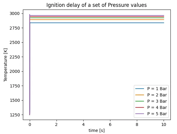
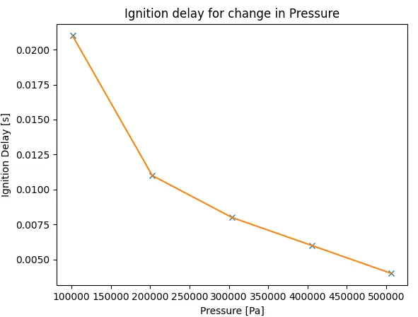
Conclusion :

1. From the first plot we can see that with increasing Pressure values in the reactor the attainable temperature also increases .
   

   Gay-Lussac's law states that the pressure of a given mass of gas varies directly with the absolute temperature of the gas when the volume is kept constant.

   Mathematically, it can be written as: `P/T=k`

2. The second plot shows that with increasing temperature the ignition delay reduces significantly .

Code 2 :

Plot the variation of Auto Ignition time of Methane with a constant pressure of 5 atm and temperature varying from 950K to 1450K.

import numpy as np
import cantera as ct 
import matplotlib.pyplot as plt

gas=ct.Solution('gri30.xml')
T_start=950
T_end=1450

P=5*101325
Temprature=np.linspace(T_start,T_end,5)
print(Temprature)
ignition_delay=[]

for T in Temprature:

	gas.TPX=T,P,{'CH4':1,'O2':2,'N2':7.52}

	r=ct.IdealGasReactor(gas)

	sim=ct.ReactorNet([r])
	time=0
	states=ct.SolutionArray(gas,extra=['time_in_ms','t'])

	for n in range(10000):

		time+=1e-3
		sim.advance(time)
		states.append(r.thermo.state,time_in_ms=time*1e3,t=time)

		if (states.T[n]<=T+400):
			
			t=(states.t[n])			

	plt.figure(1)	
	plt.plot(states.t, states.T)
	plt.legend(['T = 950K','T = 1075K','T = 1200K','T = 1325K','T = 1450K'])
	plt.title('Ignition delay of a set of Temprature values')
	plt.xlabel('time [s]')
	plt.ylabel('Temperature [K]')
	ignition_delay.append(t)

	
plt.figure(2)	
plt.plot(Temprature,ignition_delay,'x')	
plt.plot(Temprature,ignition_delay)			
plt.title('Ignition delay vs Temprature (at constant pressure [5 bar])')
plt.xlabel('Temperature [K]')
plt.ylabel('Ignition Delay [s]')			
plt.show()

Plots :

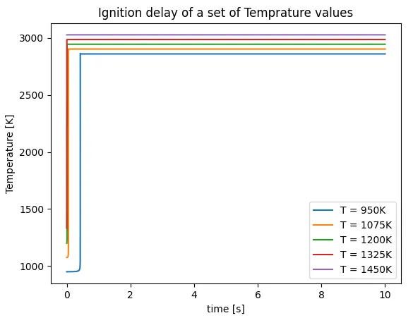
Conclusion :

1. From the first plot we can see that with increasing temperature values in the reactor the attainable temperature also increases due to combustion .
2. The second plot shows that with increasing temperature the ignition delay reduces significantly .

Code 3 :

To plot for the variation of Auto Ignition time of Methane with a constant temperature of 1250K and pressure varying from 1 to 5 atm.

&

To plot the variation of Auto Ignition time of Methane with a constant pressure of 5 atm and temperature varying from 950K to 1450K.

Briefing :

• We create a gas object and solution is used to create an instance object called gas .
• 'i' is just a loop locator ,by specifying i=0 we run the code for Temperature condition of 500K & by giving any other value other than 0 will run the code for Temperature value of 1000K.
• We create a reactor first which feeds data to the reactor network
• The for loop is used to run the code for 10 seconds by using a time step of 1e-3.
• Finally we append the values in the states variable at the end of each time step .
• Relevant plots are obtained from each case by plotting the molar concentration of each species against time.
  states.X[:,gas.species_index('species')] is used to obtain the molar concentration of our desired species from the combustion of methane .

import numpy as np
import cantera as ct 
import matplotlib.pyplot as plt

gas=ct.Solution('gri30.xml')
P=5*101325

# To choose Temprature 
i = input()

if i==0:

	T=500
	gas.TPX=T,P,{'CH4':1,'O2':2,'N2':7.52}
	r=ct.IdealGasReactor(gas)

	sim=ct.ReactorNet([r])
	time=0
	states=ct.SolutionArray(gas,extra=['time_in_ms','t'])

	for n in range(10000):

		time+=1e-3
		sim.advance(time)
		states.append(r.thermo.state,time_in_ms=time*1e3,t=time)

else:

	T=1000
	gas.TPX=T,P,{'CH4':1,'O2':2,'N2':7.52}
	r=ct.IdealGasReactor(gas)

	sim=ct.ReactorNet([r])
	time=0
	states=ct.SolutionArray(gas,extra=['time_in_ms','t'])

	for n in range(10000):

		time+=1e-3
		sim.advance(time)
		states.append(r.thermo.state,time_in_ms=time*1e3,t=time)


fig, ax = plt.subplots(3)
  
# set data with subplots and plot
ax[0].plot(states.t,states.X[:,gas.species_index('H2O')])
ax[0].set_ylabel('H20')
ax[0].set_xlabel('Time [s]')

ax[1].plot(states.t,states.X[:,gas.species_index('O2')])
ax[1].set_ylabel('O2')
ax[1].set_xlabel('Time [s]')

ax[2].plot(states.t,states.X[:,gas.species_index('OH')])
ax[2].set_ylabel('OH')
ax[2].set_xlabel('Time [s]')

# set the title to subplots
ax[0].set_title("Molar Concentration of H20")
ax[1].set_title("Molar Concentration of O2")
ax[2].set_title("Molar Concentration of OH")

# set spacing
fig.tight_layout()
plt.show()

Plots :

For T=500K

For T=1000K

Conclusion :

For H2O :

At 500K ,the molar fraction increases steadily over time .
At 1000K ,the molar fraction increases drastically within a few seconds .

For O2 :

At 500K ,the molar fraction is steady .
At 1000K ,the molar fraction decreases drastically within a few seconds .

For OH :

At 500K ,the molar fraction increases steadily over time .
At 1000K ,the molar fraction increases drastically within a few seconds .